

Welfare Effects of Unemployment Benefits when Informality is High
Abstract
We analyze for the first time the welfare effects of unemployment benefits (UBs) in a context of high informality, exploiting matched administrative and survey data with individual-level information on UB receipt, formal and informal employment, wages and consumption. Using a difference-in-differences approach, we find that dismissal from a formal job causes a large drop in consumption, which is between three to six times larger than estimates for developed economies. This is generated by a permanent shift of UB recipients towards informal employment, where they earn substantially lower wages. We then exploit a kink in benefits and show that more generous UBs delay program exit through a substitution of formal with informal employment. However, the disincentive effects are small and short-lived. Because of the high insurance value and the low efficiency costs, welfare effects from increasing UBs are positive for a range of values of the coefficient of relative risk aversion.
Introduction
Unemployment benefits (UBs) help laid-off individuals smooth consumption (insurance value), but they can also increase the duration of UB receipt and delay re-employment (efficiency costs). This tradeoff determines the welfare effects of UBs. Outside of high-income countries, the prevalence of informal employment means that individuals might receive UBs while also working informally. At the same time, the consumption drop at layoff might be higher in these contexts, especially if finding a new formal job is difficult and laid-off workers experience a high risk of poverty. Yet, while welfare effects of UBs have been studied in depth for high-income countries (Schmieder and von Wachter, 2016) fewer studies have focused on low- and middle-income countries, analyzing the insurance value (Gerard and Naratomi, 2021) or the efficiency costs of UBs (Britto 2021; Gerard and Gonzaga, 2021).1 In this paper, we jointly analyze the insurance value and the efficiency costs of UBs in a context of high informality, estimating for the first time overall welfare effects of UBs outside of a high-income country context.
Compared to other studies on UBs in both high- and middle-income countries, we additionally investigate how the possibility of working informally affects the insurance value and efficiency costs of UBs. A unique feature of our study is that we analyze data on employment, wages and consumption for all UB recipients independently from their re-employment status, including informal re-employment. Considering the nature of informal re-employment could be crucial for understanding how given levels of the welfare gains and losses of UBs materialize (see also Meghir et al., 2015; Ulyssea, 2018).2 To understand why, suppose that informal jobs are relatively easy to find and are close substitutes to formal ones. In this scenario, UB recipients have high incentives to substitute formal with informal employment, while remaining eligible for UBs and maintaining adequate consumption levels. Thus, the efficiency costs of UBs would likely outweigh their insurance value, and this effect would be larger than in labor markets where informality is less relevant. The exact opposite would apply if informal jobs are not easily accessible or do not provide wages that are comparable to those of formal jobs.
Our key result is that the welfare effects of UBs are positive and comparatively large in a context with high informality and that accounting for the nature of informal jobs is decisive to explaining this finding. The positive welfare effects stem from a pronounced consumption drop at layoff, which is between three to six times larger than existing estimates from high-income countries, and relatively small efficiency costs, which are at the lower bound of elasticity estimates from high-income countries. This is true although we document a large shift towards informal employment among UB recipients: one year after job loss, around 40 per cent of them work informally while also receiving UBs. However, the shift to informality is a response to the layoff event, while the informality response to UB generosity is relatively small. Exploiting individual-level data on informal employment is key for reconciling these findings. In particular, individuals who move to informality earn less than those who are formally re-employed and experience the largest drop in consumption. This means that informal jobs are poor substitutes of formal ones and workers seem to accept them only in the absence of better alternatives.
Our study context is the UB scheme of Mauritius, a country in the Indian Ocean with a population of 1.3 million, a level of economic development comparable to Argentina, Chile or Uruguay and 56.2 per cent of the employed population working informally. An important advantage of our setting is that it allows us to exploit a unique database, which we constructed by merging different types of individual-level administrative and survey data. The starting point are the program records of the universe of UB recipients collected at the time of job loss. We merged these with participants’ full social security biographies before and after job loss. Full social security records are also available for a large sample of the Mauritian formal labor force, corresponding to around 90 per cent of those formally employed in the country. We matched each of the two panel databases (i.e. for UB recipients and the sample of the formal labor force) with the Mauritian household survey. This means that for a representative sub-sample of the two populations, namely the sub-sample interviewed in the household survey, we additionally have information on informal employment and wages as well as household transfers and consumption.
To preview our analysis in more detail, we first study the insurance value of UBs, using a difference-in-differences (DiD) approach on the matched observations to analyze the implications of losing a formal job on consumption. We center the analysis 36 months around job loss and compare UB recipients who enter unemployment after at least 36 months of tenure in a formal job (i.e. treatment group) with a sample of individuals who constantly held the same formal job for 72 months (i.e. control group). To increase comparability between the two samples, we re-weight observations based on individual characteristics. We find that expenditures for both durable and non-durable consumption drop significantly in households of dismissed workers. Three years after job loss, total household expenditures are still 31.4 per cent lower than before dismissal and consumption expenditures are still 32.8 per cent lower. These effects are substantially larger than those observed in developed economies (Schmieder and von Wachter, 2016). Individuals who find a new informal job experience the sharpest drop in expenditures (i.e. larger than the one experienced by both those that find a formal job and those who remain unemployed).
Studying the mechanisms behind the large consumption drop, as part of the DiD-analysis we also look at the effects of job loss on employment, wages and transfers. We find that overall employment returns to pre-layoff levels two years after job loss, but there is a permanent shift in the type of job held. Even three years after job loss, those who have lost a formal job are 38.2 per cent more likely to hold an informal job. Similarly, individual monthly wages are still 48.0 per cent below the pre-layoff level three years after job loss. This is mostly because the majority of UB recipients is re-employed in informal jobs that on average pay less than formal ones, after controlling for observable characteristics. Finally, while households of laid-off individuals experience a small and transitory increase in public transfers due to the receipt of UBs, private transfers (e.g. from relatives) are largely unaffected and other forms of public transfers fail to materialize when eligibility to UBs terminates.
Subsequently, we turn to estimating the efficiency costs of UBs. We rely on the fact that benefit levels in Mauritius are subject to upper and lower bounds and adopt a regression kink (RK) analysis as in Card et al. (2015, 2017) and Landais (2015), among others. To begin with, we build on Gerard and Gonzaga (2021) who demonstrate that estimating efficiency costs in contexts of high informality only requires knowing the effect on the length of UB receipt and time until formal re-employment (i.e. we do not need to know the effect on informal employment). This is good news, as we observe these indicators for the entire sample of UB recipients from social security records. Focusing on the upper bound, we find an elasticity of length of UB receipt with respect to benefit levels equal to 0.27 (s.e.=0.11). Higher UBs also decrease the likelihood of formal employment in the months following job loss, with an elasticity of the duration without a formal job to benefit levels being equal to 0.28 (s.e.=0.14). These estimates are below the majority of those for developed economies (Schmieder and von Wachter, 2016) despite the fact that informality rates are low in those countries.
Within the RK analysis, we then study the role that informal jobs play in determining the estimated efficiency costs. To do so, we rely on the representative sub-sample of UB recipients who are also observed in the household survey. For them, we can examine the effects of UB generosity on informal employment. Close to the kink, the number of observations in the matched sub-sample is unfortunately too small for conducting the RK analysis for informal employment. For this reason, we revert to imputing informal employment for our entire sample following the literature that predicts non-durable consumption based on food expenditure (Blundell et al., 2008; Crossley et al., 2020). Specifically, we exploit that the likelihood of being informally employed changes across time (i.e., relative to the month of job loss) and that it depends on whether an individual is formally employed (where the residual category is non-employment). The results of the imputation show that we are able to replicate well the pattern of informal employment observed in the survey data. Applying the imputation to our RK analysis, we find that more generous UBs lead to an increase in informal employment. The effect is, however, small in magnitude and disappears one year after job loss. This is consistent with our earlier finding that informal jobs pay low wages, such that the incentives to move into informal employment when UBs are increased, are relatively small.
In the last part of the paper, we bring together the results from the DiD and RK analyses to estimate the welfare effects of increasing UB levels. To obtain the insurance value, we slightly readapt our DiD estimates. We follow Landais and Spinnewijn (2020) and Kolsrud et al. (2018) and estimate the flow drop in consumption around the unemployment event (i.e. at the monthly level) exploiting the fact that at the time of the interview in the household survey individuals will have spent a different number of months receiving UBs. This approach delivers an estimate of the average consumption drop at unemployment of 28.1 per cent. We then take the preferred elasticity estimates for the effects of UB levels from the RK analysis and obtain an average efficiency cost of 0.28 for a one-unit increase in UBs (i.e., the cost of the increase in benefit levels is equal to 1.28 once behavioral responses are taken into account). Comparing the insurance value with the efficiency cost, we find that welfare effects from increasing benefit levels are positive for any value of the coefficient of relative risk aversion above one. This finding suggests that in a labor market with high informality, having a formal job represents a key advantage and providing insurance against its loss is a sensible policy choice.
This paper builds on previous evidence on UB schemes in developing and emerging economies.3 Two papers examine the efficiency costs of UBs. First, Gerard and Gonzaga (2021) analyze the effects of extending UB duration in Brazil and find that longer entitlements increase length of UB receipt and delay formal re-employment, but this is mostly driven by a mechanical effect (i.e. formal jobs are difficult to find) rather than a change in incentives. Second, Britto (2021) compares the labor supply responses to the generosity of severance payments with those of an extension of UBs in Brazil and shows that the latter is more detrimental to formal labor supply in the short-run, but the effects become similar over the medium-term. A third study focuses on the insurance value: Gerard and Naritomi (2021) find that individuals increase spending when they receive lump-sum severance payments despite facing a long-run drop in earnings. We contribute to this literature by examining both the insurance value and efficiency costs of UBs for the same population.4 This allows us to compute overall welfare effects of UBs for the first time in a context of high informality.5 Additionally, we refine the existing knowledge on welfare gains and losses, even when considered independently, by observing UB recipients not only when they are formally employed, but also when they are informally employed or non-employed.6 This allows us to characterize how the availability of informal jobs affects UB receipt, re-employment, wages, consumption, and, ultimately, the welfare effects of UBs.
Having access to rich worker-level data on informality allows us to also contribute to a debate on the nature of the informal labor market. According a first stylized view, workers voluntarily choose informal employment based on their comparative advantages. A second view of informality argues that workers generally prefer formal jobs, but have difficulty accessing these. These two views on informality are no longer seen as a clear dichotomy (see La Porta and Shleifer, 2014; Meghir et al., 2015; Ulyssea, 2018). Accordingly, studies analyzing workers’ transitions show that workers move between formal and informal jobs, but that wages are higher in formal ones (Botelho and Ponczek 2011; Bosch and Esteban-Pretel 2012; McCaig and Pavcnik 2015; Díaz et al. 2018; see also the review by Ulyssea (2020)). We contribute to this literature by providing detailed evidence on the transitions of workers dismissed from a formal job. We find that formally displaced workers rapidly move to informal employment. However, they receive lower wages, have reduced consumption levels and do not return to formal jobs even long after the end of UB eligibility. This suggests that the transitions of displaced workers are asymmetric and that informal jobs are poor substitutes of formal ones.
Finally, the findings of the paper are informative to a few branches of the literature at the intersection between public and development economics. Previous studies on UBs in developed economies have found that the efficiency costs of benefit generosity are lower during downturns (Kroft and Notowidigno, 2016; Schmieder et al., 2012). This is consistent with our result of a low elasticity of the duration without a formal job to benefit levels in a context characterized by high informality rates. Although smaller than the literature on the efficiency costs of UBs, different studies have also documented drops in consumption (Ganong and Noel, 2019; Gruber, 1997; Kolsrud et al., 2018; Landais and Spinnewijn, 2020) and earnings (for a review, see Couch and Placzek (2010)) at layoff. Our estimates are among the first ones from a context of high informality and they are significantly larger than those previously obtained, which can be explained by limited self-insurance and gaps in social safety nets. Finally, previous studies have investigated the cost of public policies in contexts characterized by low enforcement capacities and high levels of non-compliance (Carrillo et al., 2017; Naritomi, 2019). We contribute to this literature by measuring for the first time non-compliance in the context of an UB scheme outside developed countries and finding relatively low efficiency costs compared to the welfare gains.
The rest of the paper is organized as follows: section 2 provides the theoretical framework for the welfare analysis; section 3 describes the institutional context and the functioning of the UB scheme in Mauritius; section 4 introduces the data sources used in the analysis and presents descriptive evidence; section 5 includes the main results from the DiD analysis on changes in consumption expenditures, labor market status, wages, and transfers around job loss; section 6 presents the imputation procedure for informality and the results from the RK analysis on the effect of benefit generosity on length of UB receipt, formal and informal employment; section 7 brings together the two main parts of the analysis to estimate the welfare effects from increasing UB levels; and section 8 summarizes and concludes.
Theoretical Framework
Insurance value and efficiency costs of UBs
Throughout the paper, we define the optimal UB level in terms of the tradeoff between the insurance value and the efficiency costs of UBs. The insurance value pertains to the role of UBs to smooth the potential drop in consumption at layoff. The efficiency costs arise due to moral hazard, whereby more generous UBs can result in delayed (formal) re-employment and longer UB receipt. We employ the job search model of Baily (1987) and Chetty (2008), as extended to labor markets with high informality by Gerard and Gonzaga (2021).
Gerard and Gonzaga (2021) show that both UB recipients who are informally re-employed and those who remain unemployed, can be treated as one group in the welfare analysis. This is based on two assumptions. First, informal workers do not pay payroll taxes and are not eligible to UBs upon layoff. Second, formally displaced workers continue receiving UBs when they are informally re-employed, as this is not detected by the authorities.7 Under these assumptions, the implications of informal re-employment are the same for welfare considerations (including public finance) as those of non-employment.8
Consider a representative worker who is laid off from a formal job in discrete time at and retires after periods. When not formally employed, the worker optimizes search efforts for a formal job (), which are normalized to equal the probability that the job search is successful. More intense job search implies a higher likelihood of finding a formal job, but also entails search costs. The same worker receives UBs (for a maximum of periods. In parallel, she can work informally to additionally earn , where is the informal wage and is the amount of informal employment provided. is chosen by the worker and entails a job effort cost of working informally; where the case of represents a non-employed UB recipient. The worker also chooses an optimal intertemporal consumption path, with consumption given by ; and has an increasing and concave utility function . Once the worker finds a formal job, she accepts it, up until earns a fixed wage of , no longer receives , and pays taxes that contribute to financing the UB scheme. She decides about an optimal consumption path () and has an increasing and concave utility function .
The social planner determines and to maximize welfare , which is given by workers’ expected lifetime utility.9 The planner’s budget constraint equals , where is the expected time spent outside of formal employment and is the expected duration of benefit receipt. Increasing UB levels requires the social planner to account for a mechanical effect, with workers receiving higher benefits throughout the duration of irrespective of any behavioral response. This is valued at the gap in marginal utilities between the non-formally employed and the formally employed. Additionally, the social planner considers the behavioral response stemming from the potential increase in the time until formal re-employment and the duration of UB receipt. Suppressing time and individual indices and normalizing terms, the marginal welfare effect of increasing amounts to (see also Schmieder and von Wachter, 2016):
|
|
(1) |
where the normalization by expresses the marginal welfare effect in terms of a one unit increase in consumption of the formally employed, while the normalization by expresses it in units of expected benefit duration. and are the elasticities of length of UB receipt and time until formal employment with respect to benefit levels, respectively. The first term on the right-hand side represents the insurance value as measured as the gap in marginal utilities between non-formally employed and formally employed workers. Empirically, we approximate the insurance value based on the flow drop in consumption after layoff, following Chetty (2008).10 The second term on the right-hand side refers to the efficiency costs defined by the behavioral response to higher UBs, both in terms of length of UB receipt and delay in formal re-employment. We estimate the parameters of Equation 1 in Sections 5 and 6 and bring them together to compute overall welfare effects in Section 7.
The role of informal jobs
Whereas informal employment does not directly enter the welfare function, having data on formal and informal employment and their implications for wages and consumption allows us to investigate the influence of informal employment on the magnitudes of the insurance value and efficiency costs. This also makes it possible to shed light on the role of informal jobs as insurance mechanisms against the loss of a formal job. Given estimates of the insurance value and the efficiency costs of UBs might be consistent with a range of different labor market dynamics and even opposite views on the role of informal employment. The two stylized views of informality assume informal employment to be the result of a voluntary choice associated with decent wages (i) or, in contrast, to be chosen out of economic necessity in the absence of better-paid alternatives in the formal sector (ii) (see Gerard and Gonzaga, 2021).
To begin with, the efficiency costs of UBs can be due to workers reacting to UB generosity by moving into informal employment as opposed to remaining unemployed. This is key to understanding whether informal jobs are readily available to laid-off individuals and the extent to which informal employment represents an additional margin of behavioral response to UB generosity. Similarly, a given positive level of the insurance value of UBs could be related to workers remaining out of employment and earning a wage in addition to receiving UBs. Alternatively, significant numbers of UB recipients could move into informal employment, but the wages they earn in these informal jobs are insufficient to preserve consumption levels.
The two stylized views on informality have similar implications in terms of the efficiency costs of UBs. Formally displaced workers may return to formal employment slowly, either because individuals do not value formal jobs more than informal ones (view (i) above) or because formal jobs are difficult to find (view (ii) above). However, these two views have opposite implications for the insurance value of UBs. If view (i) is correct, wages should be similar between formal and informal employment and informal re-employment should allow workers to cushion the consumption drop experienced at layoff. In contrast, under view (ii) wages in the informal sector should be lower than in the formal sector and informally re-employed individuals should experience large drops in consumption (Gerard and Gonzaga, 2021).
This means that a priori welfare effects of UBs can be either higher or lower in contexts of high informality. Additionally, a given level of the insurance value (efficiency costs) can be compatible with opposite views on the role of informal employment. In our analysis, we therefore begin by estimating the relevant terms that allow us to characterize Equation 1. Subsequently, we exploit our rich individual-level data to assess the role of informal jobs in determining welfare in line with the two main views presented above.
The institutional context of the Mauritian UB scheme
Mauritius is a country in the Indian Ocean with a population of 1.3 million and a median age of 36.2 years (Statistics Mauritius, 2017). The country has experienced sustained economic growth over the last decades: GDP per capita has more than doubled since the 1990s and is currently comparable to levels in Latin American countries such as Argentina, Chile and Uruguay. The Mauritian service sector accounts for the majority of employment (67.4 per cent), followed by industry and manufacturing (25 per cent) and agriculture (7.6 per cent). Despite rapid economic growth, evidence from the household survey shows that informal employment is still prevalent. An estimated 43.8 per cent of the employed population was formally employed in 2018 (i.e. employed in a job for which compulsory social security contributions to the National Pension Fund are made, as required by the relevant legislation) and this value had barely changed compared to previous years (i.e. it was equal to 44.3 in 2012, when our survey data starts).11
The current system of UBs is in place since 2009. Unemployed individuals are eligible to participate if they have been employed in a full-time job for at least six months without interruption. All reasons for job loss apply (including the expiration of a fixed-term contract), except for voluntary resignations. Eligibility is verified at the time of registration at the local Labor Office, when the dismissed worker needs to present a letter of termination of employment. Additionally, the previous employer is called upon to confirm details of the employment relation.
Conditional on meeting these criteria, laid-off individuals coming from both formal and informal jobs can enter the program. When informal workers apply, the government tries to recover social security contributions from the previous employer but fully finances the participation of the individual in the intervention if this proves impossible. In practice, however, very few informal workers apply to UBs upon layoff (i.e. they represent 20 per cent of total participants, despite accounting for roughly 70 per cent of the unemployed in the country). This is because they are both less likely to meet the program eligibility criteria and to apply conditional on being eligible, since program registration requirements (e.g. the need to present a letter of termination of employment and the requirement for the employer to confirm the dismissal) discourage their participation (Liepmann and Pignatti, 2019).
The UB received is a function of monthly gross wages earned at the time of job loss as verified from the letter of termination of employment and the unemployment duration. The amount replaced never falls below a lower bound of 3,000 Rupees (USD 184 in PPP) and never exceeds the upper bound in place in a given year (). The latter is updated annually to reflect inflation and was equal to 15,000 Rupees in 2017 (USD 920 in PPP). More specifically, UB entitlements are determined as follows:
|
|
(2) |
where is the monthly wage individual earned prior to job loss and denotes the replacement ratio in month of unemployment. In the first three months of unemployment (), the UB replaces 90 per cent of (= 0.9). This replacement ratio is reduced to 60 per cent during months 4 to 6 of unemployment (and = 0.6). Finally, during months 7 to 12 of unemployment, the replacement ratio further drops to 30 per cent of the initial wage (and = 0.3).
Upon entry into the program, participants choose among three available active labor market policies: job placement, training and reskilling, or start-up support. The vast majority opts for the job-placement option (85 per cent), but the type of support provided by the job placement services is limited. The maximum duration of UB receipt is 12 months since the time of job loss. Program eligibility ends earlier if a worker finds a new job, in theory independently from its nature. However, the two processes differ significantly between formal and informal re-employment. If the participant finds a formal job, the Ministry of Social Security detects from its records that contributions are being made for a new job and automatically de-registers the UB recipient. If the new job found is instead informal, the participant should report this information to the Labor Office that would proceed with the de-registration. However, this is difficult to enforce and there are no sanctions for failing to report a new job.
Data and descriptive evidence
Data
For the purpose of the analysis, we have obtained access to rich administrative records that we have matched with the country’s household survey. The resulting final database represents a unique source of information, allowing us to observe detailed individual and household characteristics of UB recipients independently from their re-employment status. We have combined all data sources using individual’s unique national ID numbers.
The starting point is the administrative data collected by the Ministry of Labour on the universe of UB recipients. These records are elicited at the time of registration with the program and include some basic personal characteristics (i.e. age, gender and district of residence) as well as detailed information on the elapsed job-spell (i.e. wage at job loss, tenure, reason for dismissal). This information is taken from the letter of termination of employment and the previous employer needs to confirm its accuracy. When the individual leaves the program, the date of exit is also reported. For the vast majority of UB recipients who opted for the job-placement option, we have additional information from employment centers on individual and household characteristics (e.g. educational levels, marital status, previous occupation).
Second, we rely on the social security records from the Ministry of Social Security. These records contain monthly information on individuals’ formal employment biographies. We have these full records (i.e. from the first month of contributions of the individual until December 2018) for two different populations of interest. The first is the universe of UB recipients, for which we can reconstruct all formal employment episodes before and after the unemployment spell. The second is a representative sample of the Mauritian formal labor force, obtained by appending the full employment records of those who were formally employed in a given month in all the years between 2011 and 2018.12 This second sample includes around 90 per cent of those formally employed in Mauritius during the period of analysis.13
In the rest of the analysis, we will jointly refer to these two data sources as the administrative database (or administrative records). For the sample of UB recipients, this will correspond to the panel of social security records from the Ministry of Social Security matched with information collected by the Ministry of Labour at the time of registration into the program. For this sample, we do not consider individuals who lose their job before 2011 (i.e. data from the Ministry of Labor for 2009 and 2010 presents inconsistencies, as program records were initially kept manually) and also restrict the analysis to those who enter the program by the end of 2017 (i.e. to observe them at least for one year in the social security records). We also focus on first-time program participants throughout the analysis. For the sample of the Mauritian formal labor force, the administrative database contains instead only the panel of social security records. For this sample, we restrict the time frame to between 2012 and 2018 to have a comparable period of analysis.
We have been able to match our administrative data with the Mauritian household survey administered by the National Institute of Statistics (the so-called Continuous Multi-Purpose Household Survey, or CMPHS). The merge was done at the individual and monthly level. The CMPHS is nationally representative and interviews every year around 30,000 individuals. It has a rotating panel structure, whereby a household can be interviewed four times 15 months apart (i.e. 2-2-2 rotating panel at the quarterly level). The survey has a standard content and reports information on a number of individual and household characteristics, including detailed labor market status (i.e. also covering informal employment). We have data on the CMPHS between 2012, when the survey questionnaire started asking individual ID numbers, which we use to conduct the merging, and 2018. While giving the ID number is not compulsory, the vast majority of survey respondents provide this information (i.e. 85.1 per cent of the sample).
Evaluation of the matching procedure and descriptive evidence
We now discuss the quality of the matching procedure between the administrative and survey data and present some descriptive evidence. For ease of exposition, in this part of the analysis we focus on the universe of UB recipients only.14 For this sample, we restricted the length of the administrative records to three years before and after job loss. This means that for almost all UB recipients, we have a panel of six years of social security records as well as cross-sectional information reported at the time of registration. We match this database with the household survey and find that 6.66 per cent of UB recipients are interviewed at least once in the CMPHS between 2012 and 2018. These individuals have not necessarily been observed in the CMPHS while receiving UBs, but rather in the three years before or after job loss.
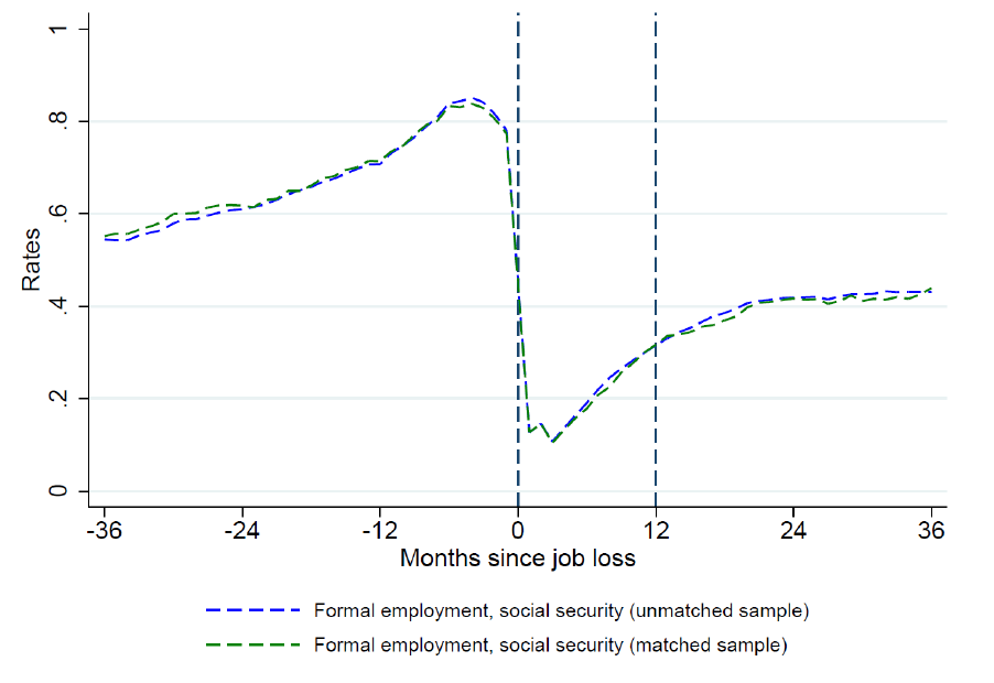
A first possible concern is the representativeness of the matched sample with respect to the overall population of UB recipients. Random sampling of the household survey should in theory guarantee this. To verify if this is the case, we compare observable characteristics between matched and unmatched individuals. We take these variables from the administrative records at job loss, so that we have information for everybody at the same point in time. Table 1 shows that there are no statistically significant differences with respect to variables related to program participation (e.g. length of receipt of UB) and characteristics of the previous job (e.g. tenure, wages). The share of individuals formally employed in a given month, as elicited from social security records, is also very similar in the two samples both before and after job loss (Figure 1). A few differences emerge with respect to individual- level characteristics (i.e. most notably, age and gender), but these are small in magnitude. Thus, the matched sample compares well overall to the universe of UB recipients.
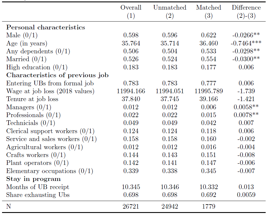
We observe that UB recipients (i.e. matched and unmatched observations) are disproportionately men (i.e. almost 60 per cent of participants). This is in line with the prevalence of male workers in the formal labor market in the country. The average age in the sample is almost 36 years and around half of the participants is married and has dependents. Individuals are generally low educated, with less than 20 per cent of UB recipients having attained at least upper secondary education. The monthly wage at job loss is on average slightly below 12,000 Mauritian Rupees, which corresponds to 736 USD in PPP and is marginally below the median wage in the country. Average tenure in the previous job is just above three years and the relative majority of participants (i.e. more than one third) was previously employed in elementary occupations. Finally, the average length of UB receipt is equal to 10.3 months and around 70 per cent of participants stay in the program for its entire duration.
A second possible concern relates to the comparability of the information provided between the two data sources. In the context of the present analysis, this is relevant particularly for variables capturing formal and informal employment. The definition of formality that we construct from the household survey is the same as the one that we observe in the administrative database. As mentioned above, this refers to the presence of job-related social security contributions to the National Pension Fund that are compulsory for the legislation. Measurement might nevertheless differ between the two sources, if survey respondents ignore their formality status or decide to misreport it (e.g. for fear that survey responses are used for auditing).
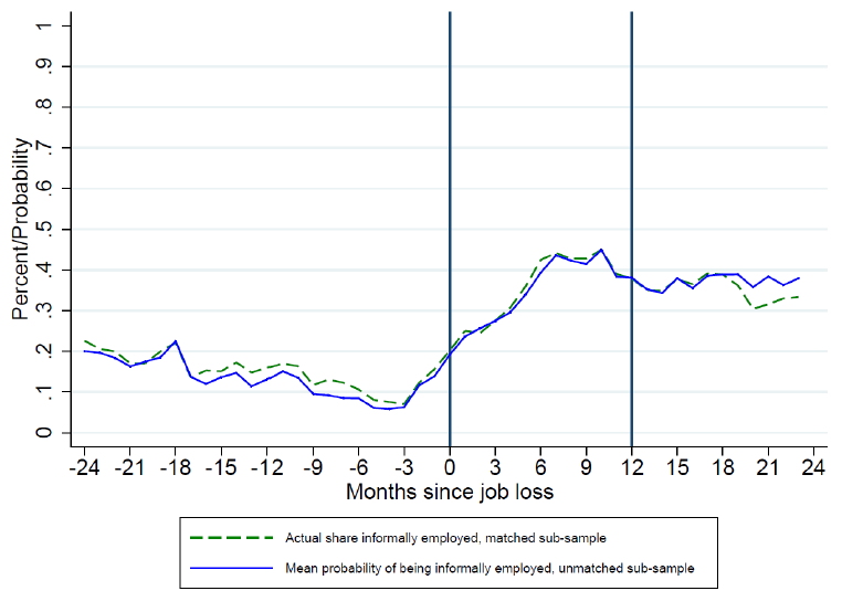
To address this concern and provide evidence on the quality of the matching, we exploit the fact that for the matched sample we have information on formal employment from both the administrative records and the household survey. Figure 2 plots the shares of individuals in our UB sample with a formal job before and after the time of job loss. The dotted green line corresponds to the dotted green line in Figure 1. It measures formality from the social security records for the matched sample and is therefore precisely observed at each point in time (i.e. independently from when the individual was interviewed in the household survey, we take the entire series of social security records). The continuous green line also reports the share of individuals who are formally employed for the matched sample, but this time measured from the household survey and using observations as repeated cross-sections (i.e. for each individual, we have a maximum of four observations over time such that different individuals are used to estimate formality rates across months). Sample size is small at the monthly level in the household survey and this leads to some noise in the series, but the figure shows that formality shares are extremely comparable between the two sources.
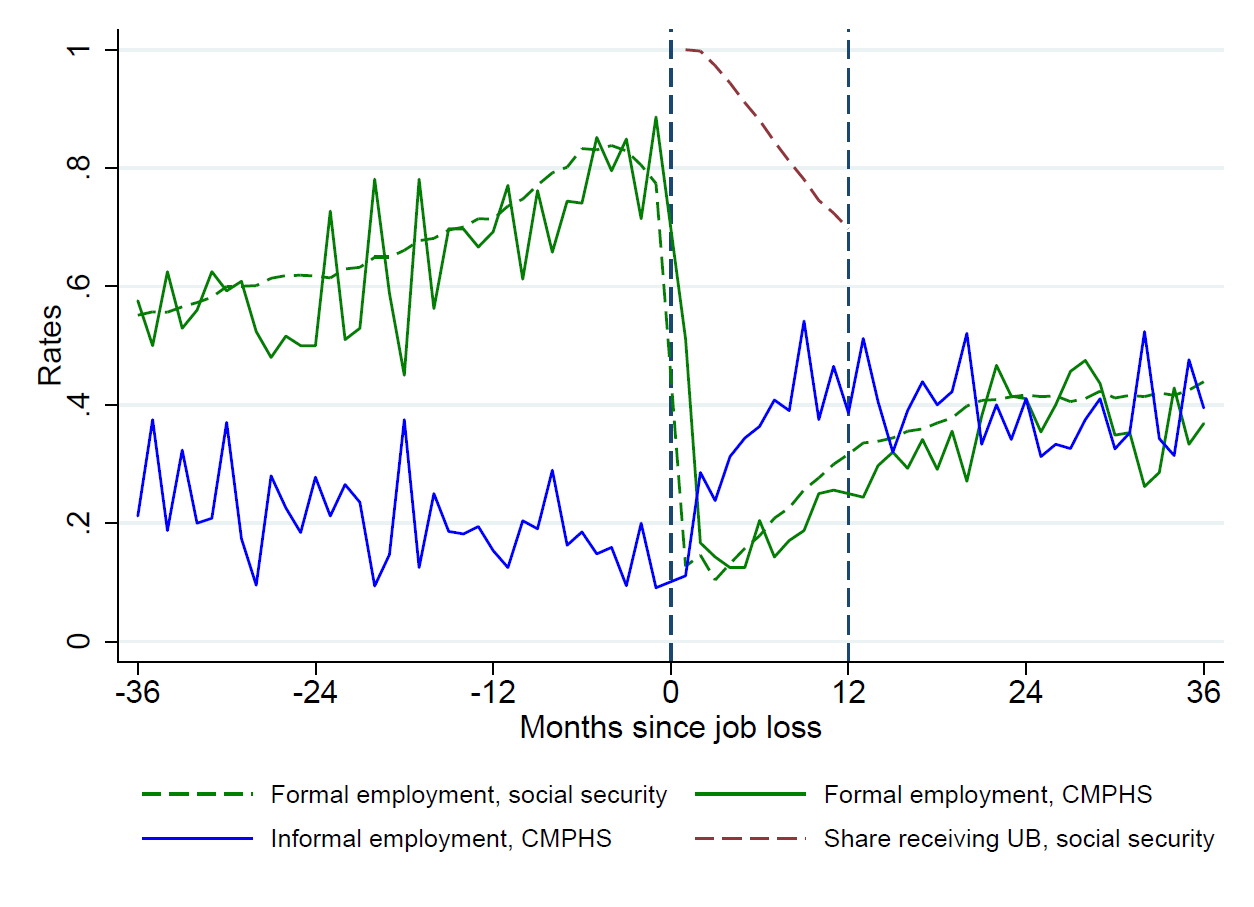
This is reassuring, because it suggests that we can credibly rely on information that is only available in the household survey (including on informal employment) to enrich the analysis.15 In Figure 2, we then plot also the informality rates for our matched sample of UB recipients (continuous blue line). A number of interesting findings emerge. First, informality is low in the period before job loss, with around 20 per cent of UB recipients holding an informal job in the year before entering the program. However, the share of individuals holding an informal job rapidly increases and settles between 40 and 50 per cent of the sample starting from six months after job loss. Around 70 per cent of UB recipients is therefore re-employed 12 months after job loss, 40 per cent informally and 30 per cent formally. Informality rates remain high even at the end of program exhaustion, when the incentives not to work formally end: three years after job loss, 40 per cent of UB recipients are still informally employed.
The evidence from the survey data shows that 12 months after job loss, only 30 per cent of program participants is without a job and is therefore still entitled to the benefit. However, we also see from the social security records that 70 per cent of UB recipients in the matched sample is still receiving UBs at that point in time (dashed red line in Figure 2). This means that 40 per cent of UB recipients are working while also receiving the benefit at the time of UB exhaustion. Therefore, the vast majority of those who find a new informal job do not report it to the Labor Office. Among the individuals who in our survey data appear to be informally re-employed in the first year after job loss, 92.5 per cent are still registered as receiving UBs in the administrative records in the same month of the survey interview. This is an important finding, as we provide the first estimates of the share of individuals working informally while receiving UBs. It implies that the level of non-compliance with program regulations is relatively high. De-registration from the program is instead automatic for individuals who find a formal job and the excessive UBs eventually transferred (e.g. due to administrative delays) are recovered.
The insurance value of UBs and underlying labor market mechanisms
We conduct a difference-in-differences (DiD) analysis centered 36 months around job loss to estimate the effects for UB recipients of losing a formal job on main outcomes of interest. The first set of outcome variables captures consumption expenditures, as this directly determines the insurance value of UBs. We then focus on a series of labor market outcomes to understand the mechanisms through which the consumption effect materializes and how the availability of informal jobs affects the insurance value of UBs.
Empirical approach
Starting from the universe of UB recipients, we restrict the sample to those who enter unemployment from a formal job, which has lasted at least 36 months before layoff as measured from the social security records.16 As common in the literature, we define a control group of individuals who never experience job loss (Gerard and Naritomi, 2021; Kolsrud et al., 2020; Landais and Spinnewijn, 2020). This group is taken from the sample of the Mauritian formal labor force for which we have full social security records, restricting the analysis to those who are reported in the same formal job for 72 consecutive months. We conduct the analysis only on observations in the treatment and controls groups that are matched in the household survey.
Imposing these restrictions, we end up with a final sample of 14,535 individuals (1,041 treated and 13,494 controls) who have been interviewed in the CMPHS in the three years around the (placebo) job loss. Table A1 in the Appendix shows selected descriptive statistics for this sample, as measured in the CMPHS. As expected, the treatment and control groups differ on a number of dimensions. In particular, UB recipients are more likely to be men and have lower educational attainments. The average age is instead similar between control and treated observations.The baseline equation takes this form:
|
|
(3) |
where is a dummy variable taking the value of one if the individual belongs to the treatment group of UB recipients; are a set of event time dummies for each quarter before and after the (placebo) job loss at ; and are calendar year and month dummies for the time in which the individual is observed in the CMPHS; and is a vector of dummies for the district of residence. We group observations at the quarterly level in order to have adequate sample size in each event time.
Given differences in observable characteristics between the treated and control groups, we re-weight observations to balance the first two moments of the covariate distributions (see Gerard and Naritomi, 2019; Landais and Spinnewijn, 2020). The re-weighting is based on the variables of sex, age, age squared as well as full sets of dummies for marital status, kinship relation and educational attainments. We apply the same re-weighting to all DiD results unless stated otherwise. Robustness tests will show that results are not particularly sensitive to the re-weighting procedure, which nevertheless increases the precision of the estimates. Standard errors are clustered at the individual level across CMPHS waves, but we do not add individual fixed effects given the relatively short length of the CMPHS panel. In the robustness tests, we will confirm that the inclusion of fixed effects is unlikely to change the results.
Main results
We now present the main results of the DiD analysis. The only coefficient we report is the one of the interaction term between the event time dummies and the dummy for UB status (corresponding to in Equation 3). We perform regressions in levels, but for the continuous outcomes we present results in relative changes by rescaling point estimates and confidence intervals by the mean in the treatment group in the quarter before job loss (i.e. which corresponds to the baseline event time). All graphs in this section will follow the same structure. In particular, we plot coefficients for the 12 quarters before and after the layoff event, which is denoted with a dashed blue vertical line. The period before job loss is included to check for parallel trends, where we expect the coefficient of interest to be non-significant. Wages and benefits will be presented gross of any taxes, but they are both subject to taxation.
A. Consumption expenditures
First, we analyze the effect of job loss on household expenditures (Figure 3). Total expenditures still remain constant in the first quarter after job loss (in line with the generous UB, which replaces 90 per cent of previous income in these months), but then rapidly decrease in the following quarters to reach a value between 20 and 30 per cent below the pre-layoff levels (panel A). Potentially because of sample sizes, the estimates for some quarters are imprecisely estimated. Yet, the overall pattern clearly indicates that the fall in expenditures persists during the three years following job loss. We observe a very similar pattern for total consumption expenditures (panel B). Additionally, we split consumption between durable and non-durable goods (panels C and D, respectively).17 We see that the drop in durable goods is larger in magnitude, but non-durable expenditures (mostly food) also fall at layoff and remain below pre-treatment trends. The result on non-durables is especially important, as it confirms that the fall in expenditures leads to a fall in consumption (see Ganong and Noel, 2019).18
Figure 3. DiD results on household expenditures
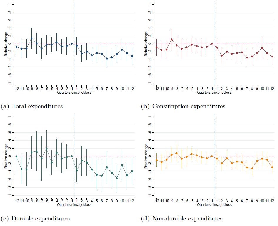
Taken together, our results indicate that the significant consumption drop implies a relatively high insurance value of UBs. Our point estimates are substantially larger than previous ones for developed economies, which are generally below 10 per cent (Ganong and Noel, 2019; Gruber, 1997; Kolsrud et al., 2018; Landais and Spinnewijn, 2020), while larger estimates have been obtained for individuals who lose their job in a recession (Schmieder and von Wachter, 2016). Our results are in line with those obtained in Brazil by Gerard and Naritomi (2021) for their sub-sample of individuals fired for cause, which is not eligible to lump-sum severance payments at layoff. Additionally, the fact that spending decreases when UB generosity falls corresponds to models where present-biased households fail to save in anticipation of a predictable income drop (Ganong and Noel, 2019; Gerard and Naritomi, 2021). At the same time, the fact that spending for non-durable also decreases confirms a consumption response to transitory income shocks (see Browning and Crossley, 2001).
To provide evidence on the role of re-employment in cushioning the drop in consumption, we look at the evolution of expenditures by re-employment status after job loss.19 Given that everybody is formally employed before layoff, this differentiation is not done for the quarters before job loss, which is why pre-treatment trends coincide and will be denoted by a unique line (Gerard and Naritomi, 2021).20 We see that the expenditure drop is the largest among those who are informally re-employed after the initial layoff (panel A in Appendix Figure A1). In contrast, individuals who are not re-employed experience similar consumption patterns as those who are formally re-employed in the two years after job loss. This suggests that individuals who remain without a job are those who can afford longer unemployment spells, while informal jobs are taken-up by credit-constrained individuals trying to prevent an even deeper fall in consumption. This could imply that informal jobs, while being relatively available compared to formal ones, provide for poor means of self-insurance. The rest of this section will further test this hypothesis and shed light on the mechanisms behind the large consumption drop, which is key to understanding what causes the high insurance value of UBs in our context.
B. Labor market status, wages and transfers
Figure 2 above has descriptively shown a large increase in informal employment following job loss. This is confirmed in the DID results on labor market status, which are reported in Figure 4. They show that the treatment group experiences a reduction in the probability of being employed (i.e. formally or informally) following job loss. However, the drop in employment is relatively small and disappears after two years (panel A).21 A similar trend is observed for unemployment (panel B) and inactivity (panel C). The relatively small drop in overall employment can be explained because the sharp reduction in the probability of being formally employed is compensated by a rapid increase in the probability of being in informal employment (panel D). This shift in the type of job held is permanent: even three years after job loss, displaced formal workers are 43.7 per cent less likely to hold a formal job and 38.2 per cent more likely to work informally. This is an important result, as we are the first to directly document such a long-term reallocation from formal to informal employment for UB recipients.22
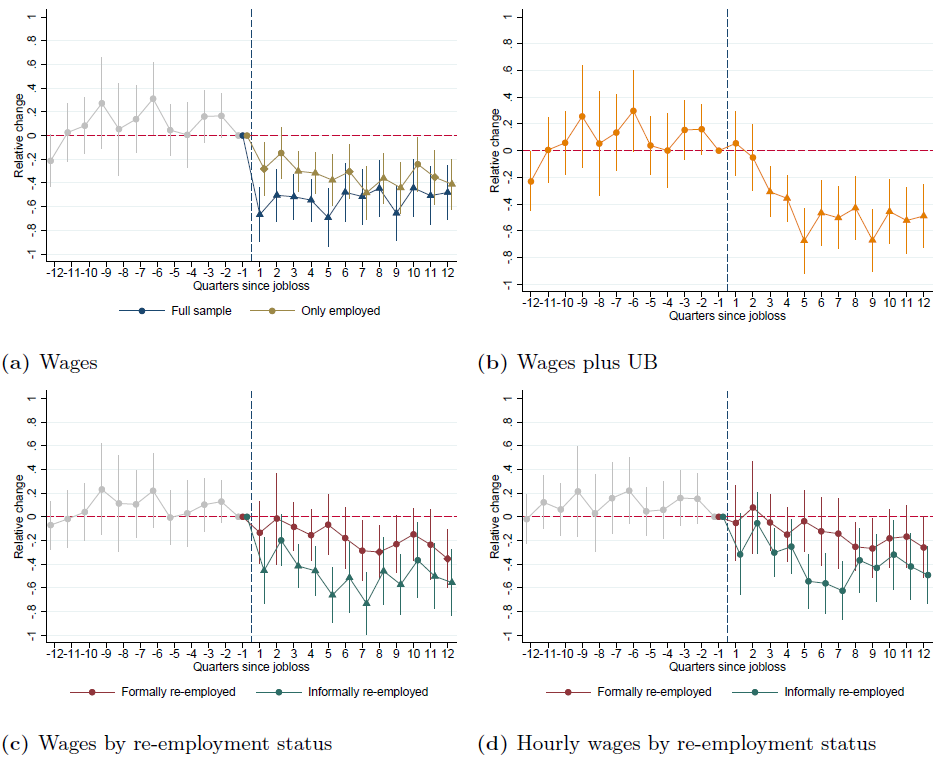
The large shift towards informal employment may explain the consumption drop documented above, provided that informal jobs are associated with inferior job characteristics. Figure 5 reports DiD results on job characteristics. We differentiate between the overall sample of UB recipients and those who find a new job after layoff and also consider the formality status of the job found. Starting with gross wages (panel A), looking at the full sample we see a decrease in monthly wages of almost 60 per cent in the year after job loss (i.e. blue line, where we assign a wage of zero to the non-employed). Wages drop also for those UB recipients who find a new job (brown line in the same figure, where the non-employed are assigned missing wages), which can be interpreted as evidence for loss of occupation, firm, or job specific human capital. The two lines converge around two years after job loss, when the majority of the laid-off individuals is back in employment. However, even three years after job loss previous UB recipients experience a wage loss of around 40 per cent.
The observed wage loss is substantially larger than previous estimates for advanced economies, which generally range between 15 and 20 per cent for prime-age workers (see the review in Couch and Placzek (2010)). As a matter of comparison, our results on wages are similar to those obtained in developed countries for displaced older workers (Chan and Stevens, 2004; Couch, 1998; Couch et al., 2009) or for individuals who lose their job in a recession (Jacobson et al., 1993). Our estimates are also larger than the few available ones for emerging and developing economies (Amarante et al., 2014), despite the fact that we also consider wages from informal work. UB receipt partially cushions the income drop at the beginning of the unemployment spell (panel B). However, benefit levels decrease sharply over time and UB eligibility ends well before wages have recovered.
As for consumption, we analyze the evolution of monthly wages for re-employed individuals by status in the new job (panel C). We find that informally re-employed individuals experience a sharper reduction in wages than those who find a new formal job (respectively, around 50 and 20 per cent wage drop on average in the three years after layoff). Differences in wages between formally and informally re-employed individuals are not driven by the fact that informal jobs require working fewer hours per week. In contrast, we see that hourly wages decline in both formal and informal jobs, but that the magnitude of the decline is larger for informal workers (panel D). The lower hourly wage indicates that informal jobs are less productive than formal ones, and that the shift towards informal employment entails a significant wage penalty (consistent with theoretical models, see Meghir et al., 2015).
The documented wage drop is before taxes and transfers. While we do not have quarterly information on the amount of taxes paid, we can investigate whether households receive transfers and if this helps alleviate the earning drop experienced at layoff. We find a small increase in total transfers after job loss (panel A of Appendix Figure A2). This comes from an increase in social security and other transfers (panels B and D, respectively), consistent with the receipt of UBs.23 At the same time, private transfers (e.g. from relatives, panel C) do not increase and other forms of public support fail to materialize after UB exhaustion. As a result, the increase in total transfers is overall small and short-lived. This is in contrast with evidence of program complementarity in developed countries, where studies have documented that individuals move to other forms of public support when eligibility to the initial transfer ends (Giupponi, 2019; Inderbitzin et al., 2016; Ye, 2020). Those who remain without a job (i.e. unemployed or inactive) benefit from the largest total transfers (panel B in Appendix Figure A1), although transfers tend to decline rapidly over time for all groups.
Figure 4. DiD results on labor market status
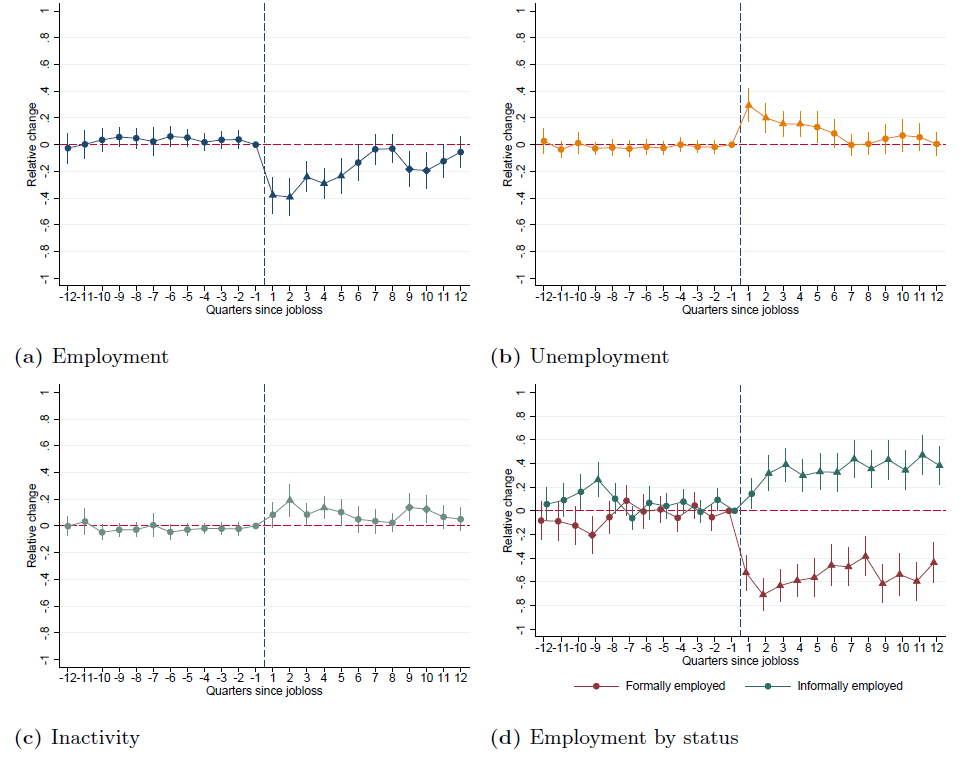
Figure 5. DiD results on job characteristics
Robustness tests
We conduct a series of tests to verify the validity of the DiD results (Appendix A). For ease of exposition, we will conduct most of these tests only for selected outcomes of interest within each outcome category (i.e. total and consumption expenditures, formal and informal employment, wages and hours worked and total and social security transfers). First, we compare our DiD results with those of a pure event study approach with no control group (Figure A3). This addresses concerns on how our control group was constructed. Second, we run the DiD specification but without re-weighting observations with the propensity score (Figure A4). This shows that the weights only increase the precision of the estimates, without drastically changing point estimates. Finally, the DiD analysis relied on repeated cross sections from the CMPHS, but for formal employment we can alternatively use the social security records and perform a panel regression. The results are almost identical using the two methods (Figure A5).
A second set of tests verifies if UB recipients anticipate job loss, which would represent a threat to identification. First, we restrict the treatment group to individuals dismissed for economic cause.24 This is done to look at more exogenous forms of job separation, in line with studies that have focused on firm closures. Results are very similar to those obtained for the overall sample (Figure A6). We then look at the probability of being registered at the public employment services (PES). The PES provide job-search support also to employed people willing to change jobs, so we should see an increase in registrations before job loss if individuals were anticipating dismissal. Instead, PES registrations go up exactly at the time of job loss (Figure A7, panel A). Similarly, we look at patterns of work absenteeism before job loss. Individuals could anticipate or even trigger the layoff by missing days of work. However, we do not find support for this hypothesis (Figure A7, panel B).
A final set of tests checks if the results by re-employment status are driven by composition effects, given that neither the timing of re-employment nor the type of job found can be taken as exogenous. First, we exploit the fact that we know the exact date of formal employment from social security records and conduct the analysis separately by groups of workers according to the month of formal re-employment. Results in Figure A8 show that all groups experience a long-term drop in wages (panel A) and expenditures (panel B), even though those who find a new job earlier do relatively better in the short-run. Second, we investigate if differences in wages between formal and informal jobs are driven by selection bias. This is done by comparing specifications which add different sets of controls. In particular, we present results, (i) with no controls (i.e. no weights), (ii) with weights obtained as in the baseline model (i.e. baseline model), and (iii) with weights obtained adding also dummies for industry (i.e. at the one digit level), enterprise type (i.e. public, private or other types) and establishment size (i.e. less than five workers, between five and nine, ten and above) (i.e. augmented specification). If selection bias was driving differences in wages, adding controls should reduce the estimated wage gap between formal and informal jobs. However, this does not appear to be the case (Figure A9).
The efficiency costs of UBs and the substitution between formal and informal employment
We now turn to analyzing the efficiency costs of UBs, which are determined by the effect of UB generosity on benefit duration and time until formal re-employment (recall Equation 1 in Section 2 above). To investigate the role of informal jobs in determining the efficiency costs, we subsequently assess whether UB generosity leads to a substitution from formal to informal employment. For effect identification we employ regression kink (RK) analysis, following Card et al. (2015, 2017) and Landais (2015), among others.
Empirical approach
A. Sample selection and empirical specification
Figure 6. Unemployment benefit entitlements in Mauritian Rupees as a function of the monthly wage at job loss and month of unemployment duration
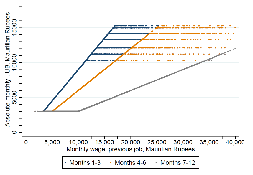
As explained in Section 3, the Mauritian UB schedule exhibits kinks at the upper and lower end, which we illustrate in Figure 6. Monthly UB entitlements decline rather strongly with time, from 90 percent of the monthly wage at job loss (during months 1-3 of unemployment), to 60 percent (months 4-6) and finally to 30 percent (months 7-12). The share of individuals for which the upper bound is binding is highest during the first three months of unemployment (equal to 13 percent, see Appendix Table B1). In contrast, the share of participants entitled only to the lower bound of the UBs peaks during the last six months of program participation (51.7 percent, Appendix Table B1). Given this distribution of participants and its implications for sample sizes, we focus on the kink at the upper bound of UB entitlements during the first three months of unemployment and the kink at the lower bound during the last six months. We additionally focus on benefit entitlements rather than benefits actually received. Entitlements are exogenous to participants’ behaviour, whereas benefits received are determined by when individuals leave the program upon re-employment (see Section 3).
Regarding the selection of our sample, we drop a small fraction of UB participants for whom the wage at job loss is implausibly small (below 1,500 Rupees) or high (top 1 percent of the real wage distribution). We also focus on individuals who worked in a formal job in the month prior to program participation.25 After imposing these restrictions, we obtain a sample of 17,791 individuals. Summary statistics are shown in Appendix Table B2 for the overall sample and for individuals in the proximity of the upper and lower bounds, respectively.
We employ a sharp RK design and estimate the following model for the upper bound:
|
|
(4) |
and for the lower bound:
|
|
(5) |
is an indicator function equal to 1 whenever an individual receives UBs corresponding to the respective bound. is a worker’s monthly wage at job loss and denotes the wage at the respective kink points. We express both variables in 2017 Mauritius Rupees and divide them by 1,000. The models are estimated for, where is the bandwidth size. In our main specifications, we use the mean squared error (MSE) optimal bandwidth of around the normalized kink points (see Calonico et al., 2017). We vary the bandwidth in robustness tests.26 The average treatment effect is given by , where is the change in slope in the relationship between the UB level and . identifies the average impact of an additional 1,000 Mauritius Rupees of UBs. For the upper bound, . Relative to initial wages, workers above this kink receive lower benefits than workers below the kink. In our analysis of the lower bound, .27 While is estimated locally, the investigation of two different kinks provides a more comprehensive understanding for different wage levels. As explained below, we show results for the upper bound in the main text and merely reference those for the lower bound, placing the corresponding results in the Appendix.
In our preferred specification, we include year and district fixed effects to account for unobservable general time trends and time-invariant regional characteristics. This is important since the upper bound changes across years and registration to the program occurs at the district level. We also investigate how the inclusion of additional covariates affects our results. These include age and its square, marital status (captured by 4 categories), the number of dependents (3 categories) and educational attainment (3 categories). These covariates should not substantially affect our estimates provided that the identifying assumptions of the RK analysis are satisfied.
B. Imputation of informal employment
In contrast to all other outcome variables analyzed in this section, we observe informal employment only for the sub-sample of program participants we could match with the survey data, which means that sample sizes in the proximity of the kinks are very small. Based on the matched sub-sample, we thus revert to imputing the probability for individuals in the unmatched sub-sample to be informally employed in a given month. We build on the literature that started with Blundell et al. (2008) and predicts non-durable consumption based on food expenditure (see also Browning et al., 2003; Blundell et al., 2004; Attanasio et al., 2015; Kaplan et al., 2020). This methodology distinguishes between time-varying proxy variables (i.e., the main explanatory variables in the imputation regression) and variables that serve as controls. Both types of variables need to be available for the matched and unmatched sub-samples.
Our imputed outcome variable, , is defined as the probability for an individual to be informally employed in month around job loss. We focus on this two-year window to show pre-treatment trends and dynamics over time. Two empirical observations guide our choice of proxy variables. First, the likelihood of being informally employed changes around job loss. It is low in the months before job loss, but then significantly increases with time spent in the program (recall the discussion of Figure 2 above). Second, the likelihood of being informally employed in a given month does not increase for those who hold a formal job, an information that we observe for our entire sample (where the residual category is non-employment). Therefore, we include as proxy variables a dummy variable , capturing whether an individual worked formally in a given month according to social security records, month since job loss fixed effects , and full interactions between these two sets of variables.28 We additionally include demographic control variables, thereby accounting for any observed differences between matched and unmatched sub-samples in terms of age, gender, marital status, number of dependents or education (see Table 1 above).29 The imputation regression is then estimated for individuals we could match with the household survey and takes the following form:
|
|
(6) |
The results for this regression are shown in Appendix Table B3. Its R-squared is 0.26 and the partial R-squared pertaining to the proxy variables is 0.16, which is reasonably high given the relatively sparse set of variables. We next predict the likelihood of being informally employed in a given month for the unmatched observations. Figure 7 shows that we are able to replicate well the pattern of informal employment around job loss. However, since this prediction is naturally associated with imprecision in the imputed outcome variable, we need to account for the fact that the usual standard errors of the coefficients relating UBs to informal employment (i.e., of in equations 4 and 5) are too small. Moreover, due to non-classical, or Berkson type, measurement error in the dependent variable, these coefficients are downward biased. We correct for both phenomena relying on the procedure and Stata routine of Crossley et al. (2020) for our RK results on informal employment.
Figure 7. Share informally employed in a given month around job loss, actual versus imputed
Assessment of the identifying assumptions
The RK methodology hinges on two identifying assumptions. First, the density and the partial derivative of the density of the assignment variable are assumed to evolve smoothly around the kink. Intuitively, this rules out that observed changes in the outcomes of interest are generated by sample selection. Figure 8 displays the number of observations in each bin of the wage distribution at layoff, normalized by the wage at the upper bound for a bin size of 0.0125. Panel A shows the entire distribution of participants, while panel B focuses on observations close to the upper bound according to an MSE-optimal bandwidth. The figure shows no sign of discontinuity around the kink, which is confirmed by the McCrary (2008)-test. We also test for a possible discontinuity of the partial derivative of the density as in Landais (2015) and cannot reject the null hypothesis of no discontinuity (see Figure 8).30
Figure 8. Probability density function of the running variable around the upper bound
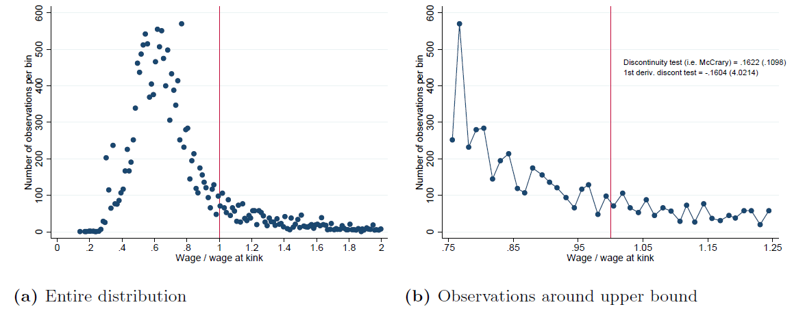
Lack of sorting at the upper bound is coherent with the institutional setting faced by UB recipients. The upper bound has changed every year during the period of analysis and is computed as 90 per cent of the threshold at which social security contributions are capped. Identifying these values is complex and participants would also need to optimize based on the presumed schedule that will apply when they can expect to be dismissed. In contrast with this understanding, there is evidence of sorting at the lower bound (see Appendix Figure B1). Although we cannot directly test the reasons behind this, the lower bound was binding throughout the study period for individuals whose initial wage was equal to 10,000 Rupees. This is a round amount, where a mass of individuals is naturally concentrated. Coherently, we see similar discontinuities for placebo kinks at pre-layoff wages of 8,000 and 12,000 Rupees.
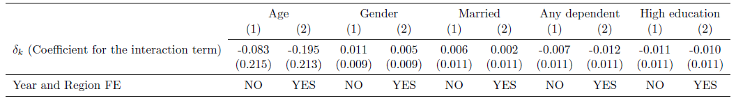
The second assumption needed for RK is that the marginal effect of the assignment variable on the outcomes of interest is smooth at the kink. Figure 9 shows that observable individual-level characteristics measured at the time of job loss (i.e. gender, age, marital status, presence of dependents and educational attainments) evolve smoothly around the kink at the upper bound. We confirm this result by running regressions in the form of Equation 4, but using the covariates as dependent variables (Table 2). Finally, we estimate the main outcome of interest (i.e. length of UB receipt) based on pre-determined covariates (as in Britto, 2016; Ye, 2020).31 Panel E of Figure 9 shows that the predicted length of UB receipt evolves smoothly around the kink. Instead, the presence of bunching at the lower bound implies that some of the covariates do not evolve smoothly around that kink (i.e., gender and age, see Appendix Figure B2 and Table B4). This leads us to focus on the upper bound in the rest of the analysis and present results for the lower bound only as a matter of comparison.
Figure 9. Evolution of covariates around the upper bound
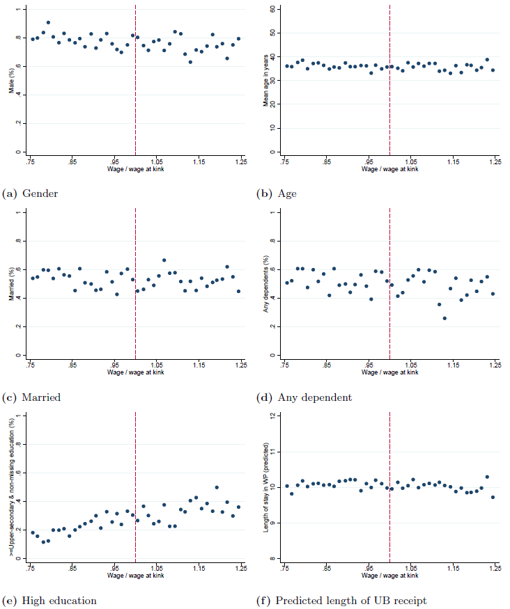
Table 2. Smoothness of covariates at the upper bound
Main results
A. Benefit duration and time before formal re-employment
As a first outcome, we analyze how increased UBs impact the duration of benefit receipt for individuals affected by the upper bound of the benefit schedule. The emerging pattern stands in clear contrast to the smooth evolution of covariates and the predicted outcome presented above. The scatter bin plot for length of UB receipt shows a change in the slope around the kink point (Figure 10). To the left of the kink, where benefits amount to 90 per cent of previous earnings, we observe a positive relationship between underlying wages and UB duration. That relationship becomes flat to the right of the kink, where UBs are capped at the maximum level. This suggests that replacement rates below 90 per cent induce individuals to exit the program faster and to receive UBs for a shorter time. Results are similar without controls (panel A) and with the inclusion of year and district fixed effects (panel B, which plots regression residuals).
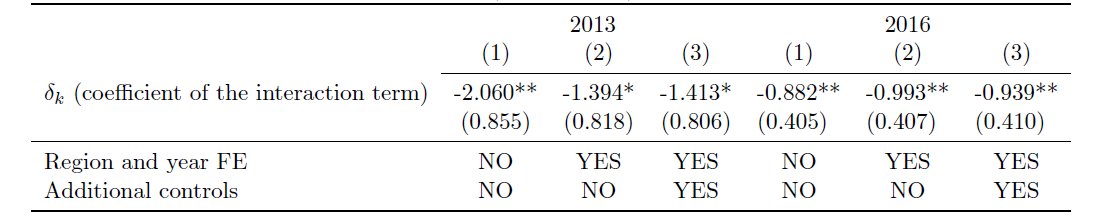
The RK-results in Table 3 corroborate this finding. Our preferred specification includes only district and year fixed effects and indicates that benefit receipt increases by 0.184 months due to a 1,000 Rupee (USD 61 in PPP) increase in the UB level (column 2). The effect is virtually the same when additional control variables are added (column 3). It is larger in the specification without any control variables (column 1), which demonstrates the importance of accounting for district and year. The elasticity corresponding to our preferred specification equals 0.27 (s.e. 0.11). Although they must be interpreted with some caution, we find similar effects at the lower bound (see Figure B3 and Table B5).32 In comparison, Schmieder and von Wachter (2016) report a median elasticity of UB receipt to benefit levels of 0.30 for studies in the US and Europe (authors’ calculation based on Table 2 in their review).33 Our estimates are thus below the median of those typically found for high-income economies, despite informality being low in those countries.
Figure 10. Scatter bin plots for the duration of UB receipt (in months) at the upper bound
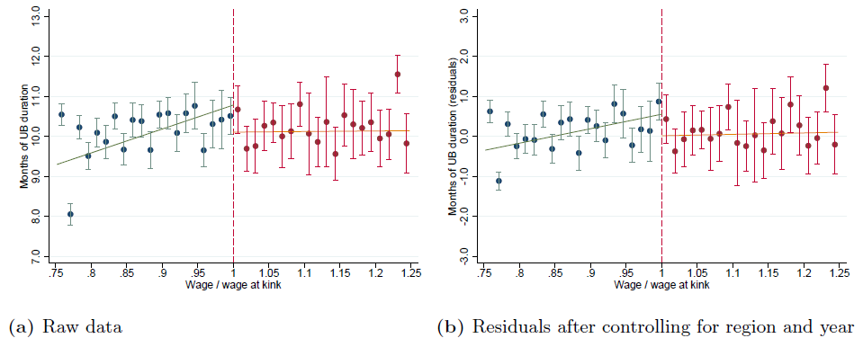
Notes: The figures show mean values and 90 per cent confidence intervals of UB receipt in months per bin of size 0.0125 around the normalized kink point, based on raw data (panel A) and after controlling for region and year fixed effects (panel B). The MSE-optimal bandwidth of 0.248 was used. Linear models were fitted on both sides and independently of the choice of bin size; i.e., all programme participants are weighted equally in the linear fits. The figure might seem to be influenced by the presence of outliers at the two extremes of the bandwidth. In reality, their exclusion would change the slope of the lines on the two sides of the cutoff while still maintaining a change in slope at the cut-off. The robustness tests will check the sensitivity of the results to bandwidth choice.
Table 3. RK-results for the duration of receiving UBs (months), upper bound
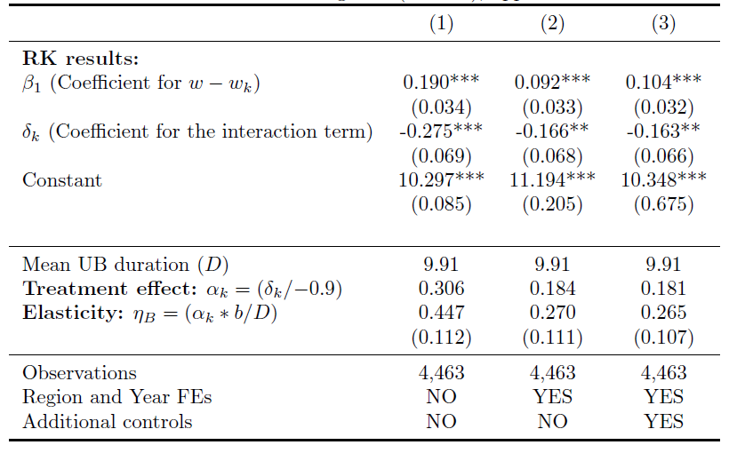
Figure 11. Hazard rate of formal employment and share of UB participants finding a formal job in each month after job loss
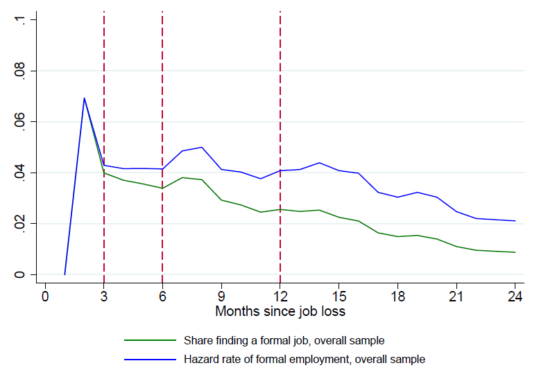
UB efficiency costs also depend on the total time spent out of employment, independently from the length of benefit receipt. In this regard, we follow Gerard and Gonzaga (2021) who show that, even in a context characterized by high informality, efficiency costs arise only from the effect of UB generosity on delayed formal (but not informal) re-employment. Using our preferred specification at the upper bound, we obtain elasticity estimates of the duration out of a formal job with respect to benefit levels of 0.28 (s.e. 0.14) when we cap formal re-employment at one year after job loss and 0.21 (statistically not-significant) when we cap it at two years. These estimates are substantially lower than those generally found in developed economies (the median estimate is equal to 0.57 in the review by Schmieder and von Wachter (2016)). This can be explained by the fact that hazard rates of formal employment remain low in our sample even after individuals lose benefit eligibility (Figure 11), while they spike right after UB exhaustion in other contexts (Card et al., 2007).34
B. Formal and informal employment
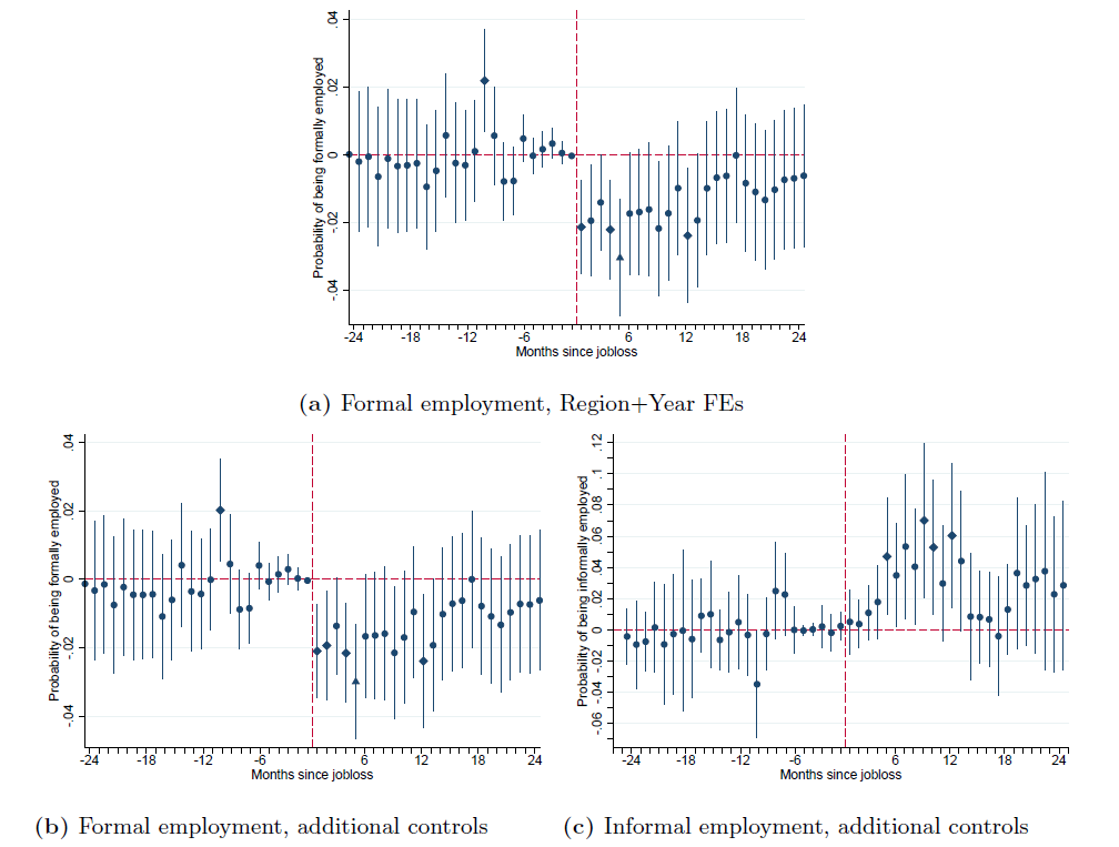
We next analyze formal and informal employment responses to UB generosity. To show dynamics over time and capture pre-treatment trends, we assess each month separately in a two-year window around job loss.35 In Panels (a) and (b) of Figure 12, we compare the RK-results for formal employment at the upper bound with few and additional control variables, corresponding to specifications in columns (2) and (3) in Table 3. Here, the outcomes are dummy variables equal to one whenever an individual was formally employed in a given month as observed in the social security data. We find that higher UBs have a negative effect on formal employment in the 12 months after job loss, with seven of the twelve estimated coefficients being statistically significant at least at the ten per cent level. The effect is strongest in the fourth month after job loss, where our estimate indicates that a 1,000 Rupee increase in UBs decreases formal employment by 3.0 percentage points (the share formally employed in that month is 20 percent). The negative effect on formal employment does not persist in the second year after job loss. These findings are corroborated by the neutral pre-treatment trend and results are very similar with few or additional controls.
In Panel (c) of the same figure, we analyze informal employment. As explained in Section 6.1, the outcome variables are the imputed probabilities for individuals to be informally employed in a given month. We directly include all control variables to account for differences between the samples that we use in our imputation procedure (see the discussion in Section 6.1). We find that higher UBs increase the likelihood to be informally employed. Compared to formal employment, the effect on informality occurs with a time-lag and becomes apparent in months 4 to 12 after job loss (after correcting standard errors, eight out of these nine coefficients are statistically significant at least at the ten per cent level). The effect on informality is largest in the eighth month after job loss, where a 1,000 Rupee increase in UBs is estimated to increase the likelihood of being informally employed by 7.0 percentage points (the imputed share of individuals informally employed equals 42 percent in that month). Again, the effects on informality do not persist beyond the first year after job loss and are corroborated by a neutral pre-treatment trend.
Comparing the formal and informal labor supply effects, up until the third month after job loss, we only observe the negative effect on formal employment. However, from months four to 12 we see a strong increase in informal labor supply. That is, we find that higher UBs entail a substitution from formal to informal employment. Our estimated net employment effect (i.e. formal plus informal) appears to be non-negative, although we refrain from directly comparing coefficients on formal and informal employment due to differences in the outcome variables (i.e. dummy for formal employment and probability for informal employment). These results represent the first evidence of substitution of formal with informal employment due to an increase in UB levels in emerging and developing economies. However, they are consistent with findings from studies that have documented this type of substitution as a result of the expansion of social protection schemes (Camacho et al., 2014) or the receipt of cash transfers (Bergolo and Cruces, 2021). Similar results were also obtained in Brazil for an increase in UB duration by Britto (2021) through an indirect matching of administrative and survey data as well as by Gerard and Gonzaga (2021) using descriptive survey evidence.36
Figure 12. RK-results for the probabilities of being formally and informally employed in a given month around job loss, upper bound
Finally, we replicate the results discussed in this section for the lower bound (see Appendix Figures B5 and B6). While these must be interpreted with caution, it is reassuring that after job loss they are qualitatively similar to those found at the upper bound.37
Robustness tests
We now present robustness tests to confirm the validity of the RK results. For ease of exposition, in the text we focus on the outcome of UB receipt and refer to our preferred specification (i.e. with only year and district dummies as controls), but results for other outcomes of interest can be consulted in the Appendix (Appendix Figure B7 and Tables B6 and B7).38 First, we test the sensitivity of the results to the bandwidth choice. Results presented so far were obtained with the MSE-optimal bandwidth, which represents an improvement of earlier solutions (see, Imbens and Kalyanaraman (2012) and Calonico et al. (2014)). We now present results for all bandwidth from 0.05 to 0.35 (see Appendix Figure B8). The MSE-optimal bandwidth (equal to 0.248) is denoted by a long-dashed vertical line; while the Coverage Error Rate (CER) optimal bandwidth is denoted with a short-dashed red line and is equal to 0.142. In line with expectations, estimates are larger in magnitude but less precisely estimated as we get closer to the cutoff. It should also be noted that the RK design performs poorly with small samples relative to regression discontinuity methods (see Landais, 2015). Results are in any case significant at conventional levels for a range of choices in the vicinity of both the MSE- and CER-optimal bandwidths.
A second concern relates to the choice of the polynomial order. Results presented so far have been obtained with a linear specification. There is a debate in the literature on how to identify the optimal model in analyses with regression discontinuities or kinks (Pei et al., 2020), generally favoring lower polynomial orders (Gelman and Imbens, 2019). We observe that the Aikake Information Criterion (AIC) marginally prefers the quadratic specification, while the Bayesian Information Criterion (BIC) strongly favors a linear model. The main results on length of UB receipt are generally confirmed in specifications that use the two preferred polynomial orders (although they partially lose significance in some of the quadratic specifications), while they change sign and lose statistical significance in the cubic specification (see Appendix Table B8). This sensitivity is not particularly worrying given the discussion in the literature, and the results of the AIC and BIC tests, and is common to a number of studies that adopt RK methods (see Böckerman et al., 2018; Manoli and Turner, 2018; Ye, 2020).
A final set of tests refers to the possible functional dependence between the forcing variable and the outcome of interest. We assume that this relationship is smooth at the kink, but it could be kinked or quadratic. First, we aim to detect non-parametrically the presence of a kink by looking at the breakpoint that minimizes the residual sum of squares. Appendix Figure B9 plots the for the model with length of UB receipt as the dependent variable for different kink points. It shows that the increases sharply in the proximity of the true kink. We also run RK estimates with a placebo forcing variable. The challenge is to identify a meaningful placebo (i.e. a proxy of previous earnings) that is at the same time not too correlated with wages at job loss. We follow Landais (2015) in using re-employment wages for formal employment. We do not find any treatment effect in this placebo test (Appendix Table B9). Finally, we exploit variations in the location of the kink in absolute terms over time (see Figure 6) in a double difference RK design (DD-RK). The intuition is to compare slope changes in the relationship between the outcome of interest and the forcing variables between years when the kink was in place at that point of the wage distribution and years in which the kink was somewhere else.39 Appendix Table B10 shows that the DD-RK estimates confirm the results of the analysis, while being larger in magnitude.
Welfare analysis
In the last part of the paper, we bring together the results from the DiD and RK analyses to derive the marginal welfare effect of increasing UB levels. We follow the sufficient statistics approach of Baily (1978) and Chetty (2006, 2008), as adapted by Gerard and Gonzaga (2021) to contexts of high informality and presented in Section 2. We have already estimated most of the terms in Equation 1 (recall that the insurance value is approximated by the flow drop in consumption, rescaled by the coefficient of relative risk aversion, Chetty (2008)).
Starting with the insurance value, we have documented in Section 5 a sharp and persistent drop in consumption following job loss. However, those results were obtained for the overall sample of UB recipients. To consistently estimate the insurance value and efficiency cost for the same underlying population, we replicate the main findings of the DiD analysis for the sub-sample in the proximity of the upper bound. Appendix Figure A10 shows that the main results continue to hold for individuals around the kink. However, we want to retrieve a higher frequency measure of the drop in consumption. To this end, we follow Landais and Spinnewijn (2020) and Kolsrud et al. (2018) and exploit the fact that those interviewed in the CMPHS in the year following job loss have spent a different number of months in unemployment at the time of the interview. Restricting the analysis to individuals around the upper bound, we augment the DiD specification (Equation 3 in Section 5.1) by including an additional term for the number of months spent in unemployment at the time of interview, to obtain an estimate of the consumption drop at the monthly level.40 This yields an estimated drop in consumption equal to 0.281 (s.e. 0.126), which is very similar to what we discussed in Section 5.2 for the sample of all UB recipients, but again larger than most estimates from advanced economies.
Turning to the efficiency costs, we take our preferred estimate of elasticity of benefit duration (i.e. 0.27) and time for formal re-employment (i.e. 0.28). These are local estimates stemming from our analysis of the upper bound and can be directly used to estimate the efficiency costs as defined in Equation 1. and are observed in the sample as the mean duration in the UB program and the mean time before formal re-employment, respectively, for the population around the upper bound (equal to 9.91 and 14.93, see column (2) in Appendix Table B2). Finally, we follow Landais (2015) and Gerard and Gonzaga (2021) in approximating with the share of UB recipients per formal employee in the country.41 This leads us to an estimate of 0.283 for the behavioral cost, meaning that a one unit increase in UBs will generate a public cost of 1.283 once behavioral responses are taken into account.42 This is lower than most estimates for advanced economies (Schmieder and von Wachter, 2016). However, our results are very similar to those obtained by Gerard and Gonzaga (2021) in Brazil for an increase in UB duration. This confirms that efficiency costs might be lower in emerging and developing economies, despite higher informality rates. This finding can be rationalized by the fact that informal jobs pay comparatively low wages and that finding a formal job is difficult.
Table 4. Welfare effects from increasing UB levels
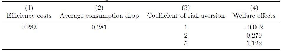
In Table 4, we present our estimates of the welfare effects of an increase in UB levels. The results show that welfare effects are close to zero for a coefficient of relative risk aversion equal to one, and positive for any value above one. While there is debate in the literature on the value of the coefficient of risk aversion, most studies generally take one as the lower bound (Chetty and Szeidl, 2007; Schmieder and von Wachter, 2016). This implies that an increase in benefit levels would likely be welfare improving in our context. Our welfare estimates are in any case more favorable than those obtained in previous studies in advanced economies (i.e. the median estimate for is equal to 0.21 in the review by Schmieder and von Wachter (2016)), whereas no previous estimates exist for low- and middle-income economies.
Conclusion
This paper analyzes the welfare effects of UB generosity in a context of high informality, where it is a priori unclear whether the presence of informal jobs increases or decreases welfare gains. We provide one of the first estimates in low- and middle-income countries of the behavioral response to UB generosity and of the drop in consumption at layoff, while bringing together these elements for the first time. Having access to data on employment, wages and consumption of formal and informal workers, we characterize both the efficiency cost and the insurance value of UBs in terms of the substitutability between formal and informal jobs. This is important to inform a debate on the nature and role of informal jobs.
Our results reveal that the detrimental effects of job loss are large in magnitude and persist over time, while the response to UB generosity are relatively small and rapidly disappear. As a result, we find that efficiency costs are below the median of existing estimates from high-income economies while our estimate of the insurance value of UBs is substantially larger than previous results. This can be interpreted by the fact that displaced workers move to informal employment out of necessity, having to accept lower-paying jobs. This, in turn, generates a large drop in consumption, which persists over time as individuals fail to return to formal employment. Welfare effects of UB generosity are therefore positive and comparatively large.
The findings of the paper have important policy implications, as they show that the unintended consequences of UB schemes in low- and middle-income countries might have been overstated and their benefits sometimes overlooked. UB schemes are still absent in around half of all middle-income and in most low-income countries (Asenjo et al., 2019), partly due to a general understanding that efficiency costs would be substantially higher in contexts of high informality (Duval and Loungani, 2019; Robalino et al., 2009). Our empirical results, however, suggest otherwise. In a context characterized by high informality, a formal job gives workers a key economic advantage and its loss represents an event from which it is difficult to recover. Providing UBs to formally displaced workers is therefore a sensible policy option, with the welfare gains largely outweighing the efficiency costs.
Acknowledgements
We would like to thank Janine Berg, Sandra Black, Richard Blundell, Antonio Cabrales, Lucia Corno, Christian Dustmann, Giacomo de Giorgi, Verónica Escudero, François Gerard, Rafael Lalive, Thomas Le Barbanchon, Peter Levell, Attila Lindner, Santo Milasi, Dana Müller, Tobias Müller, Michele Pellizzari, Giorgio Presidente, Jesse Rothstein, Uta Schönberg, Domenico Tabasso, Michela Tincani, Alessandro Tondini, Gabriel Ulyssea as well as participants at presentations at AIEL, EALE, ESPE, IAFFE, IFS, ILO, SSES and the University of Geneva for helpful comments. We are also very grateful to the staff at the Ministry of Labour, Human Resource Development and Training in Mauritius, who provided access to part of the data used in the analysis, coordinated the data gathering process with other institutions in the country and clarified many policy details. Chiara Lacava and Olivier Lenoir provided excellent research assistance. Clemente Pignatti acknowledges financial support from the Swiss National Foundation through grant P1GEP1\_191322. The responsibility for opinions expressed in this article rests solely with its authors, and publication does not constitute an endorsement by the International Labour Office of the opinions expressed in it. All remaining errors are ours.
References
Amarante, V., R. Arim, and A. Dean (2014). The Effects of Being Out of the Labor Market on Subsequent Wages: Evidence for Uruguay.
Asenjo, A., V. Escudero, H. Liepmann, C. Pignatti, and D. Tabasso (2019).
Attanasio, O., E. Hurst, and L. Pistaferri (2015). The Evolution of Income, Consumption, and Leisure Inequality in the United States, 1980-2010. In C. D. Carroll, T. F. Crossley, and J. Sabelhaus (Eds.),
Azuara, O. and I. Marinescu (2013). Informality and the expansion of social protection programs: Evidence from Mexico.
Baily, M. N. (1978). Some aspects of optimal unemployment insurance.
Böckerman, P., O. Kanninen, and I. Suoniemi (2018). A kink that makes you sick: The effect of sick pay on absence.
Bergolo, M. and G. Cruces (2014). Work and tax evasion incentive effects of social insurance programs: Evidence from an employment-based benefit extension.
Bergolo, M. and G. Cruces (2021). The Anatomy of Behavioral Responses to Social Assistance When Informal Employment Is High.
Blundell, R., L. Pistaferri, and I. Preston (2004). Imputing Consumption in the PSID using Food Demand Estimates from the CEX. Institute for Fiscal Studies, Working Paper WP04/27.
Blundell, R., L. Pistaferri, and I. Preston (2008). Consumption Inequality and Partial Insurance.
Bosch, M. and R. M. Campos-Vazquez (2014). The Trade-Offs of Welfare Policies in Labor Markets with Informal Jobs: The Case of the “Seguro Popular" Program in Mexico.
Bosch, M. and J. Esteban-Pretel (2012). Job creation and job destruction in the presence of informal markets.
Bosch, M. and N. Schady (2019). The effect of welfare payments on work: Regression discontinuity evidence from Ecuador.
Botelho, F. and V. Ponczek (2011). Segmentation in the Brazilian Labor Market.
Britto, D. (2021). The employment effects of lump-sum and contingent job insurance policies: Evidence from Brazil.
Browning, M. and T. F. Crossley (2001). Unemployment insurance benefit levels and consumption changes.
Browning, M., T. F. Crossley, and G. Weber (2003). Asking Consumption Questions in General Purpose Surveys
Calonico, S., M. Cattaneo, M. Farrell, and R. Titiunik (2017). rdrobust: Software for regression discontinuity design.
Calonico, S., M. D. Cattaneo, and R. Titiunik (2014). Robust nonparametric confidence intervals for regression-discontinuity designs.
Camacho, A., E. Conover, and A. Hoyos (2014). Effects of Colombia's social protection system on workers' choice between formal and informal employment.
Card, D., R. Chetty, and A. Weber (2007). The spike at benefit exhaustion: Leaving the unemployment system or starting a new job?
Card, D., D. Lee, Z. Pei, and A. Weber (2015). Inference on Causal Effects in a Generalized Regression Kink Design.
Card, D., D. Lee, Z. Pei, and A. Weber (2017). Regression Kink Design: Theory and Practice
Carrillo, P., D. Pomeranz, and M. Singhal (2017). Dodging the taxman: Firm misreporting and limits to tax enforcement.
Chan, S. and A. Stevens (2004). How does job loss affect the timing of retirement?
Chetty, R. (2006). A general formula for the optimal level of social insurance.
Chetty, R. (2008). Moral Hazard versus Liquidity and Optimal Unemployment Insurance.
Chetty, R. and A. Szeidl (2007). Consumption Commitments and Risk Preferences.
Couch, K. A. (1998). Late Life Job Displacement.
Couch, K. A., N. A. Jolly, and D. W. Placzek (2009). Earnings losses of older displaced workers: A detailed analysis with administrative data.
Couch, K. A. and D. W. Placzek (2010). Earnings losses of displaced workers revisited.
Crossley, T. F., P. Levell, and S. Poupakis (2020). Regression with an Imputed Dependent Variable. Institute for Fiscal Studies, Working Paper W20/25.
Díaz, J. J., J. Chacaltana, J. Rigolini, and C. Ruiz (2018). Pathways to Formalization: Going beyond the Formality Dichotomy. IZA Discussion Paper No. 11750.
Duval, R. A. and P. Loungani (2019). Designing Labor Market Institutions in Emerging and Developing Economies: Evidence and Policy Options. IMF StaffDiscussion Note 19/04.
Galasso, E. and M. Ravallion (2004). Social protection in a crisis: Argentina's plan Jefes y Jefas.
Galiani, S. and P. J. McEwan (2013). The heterogeneous impact of conditional cash transfers
Ganong, P. and P. Noel (2019). Consumer spending during unemployment: Positive and normative implications.
Garganta, S. and L. Gasparini (2015). The impact of a social program on labor informality: The case of AUH in Argentina.
Gelman, A. and G. Imbens (2019). Why high-order polynomials should not be used in regression discontinuity designs.
Gerard, F. and G. Gonzaga (2021). Informal Labor and the Efficiency Cost of Social Programs: Evidence from the Brazilian Unemployment Insurance Program.
Gerard, F. and J. Naritomi (2021). Job Displacement Insurance and (the Lack of) Consumption-Smoothing.
Giupponi, G. (2019). When Income Effects are Large: Labor Supply Responses and the Value of Welfare Transfers. Working Paper.
González-Rozada, M. and H. Ruffo (2016). Optimal Unemployment Benefits in the Presence of Informal Labor Markets.
Gruber, J. (1997). The consumption smoothing benefits of unemployment insurance.
ILO (2021).
Imbens, G. and K. Kalyanaraman (2012). Optimal Bandwidth Choice for the Regression Discontinuity Estimator.
Inderbitzin, L., S. Staubli, and J. Zweimüller (2016). Extended unemployment benefits and early retirement: Program complementarity and program substitution.
Jacobson, L. S., R. LaLonde, and D. Sullivan (1993). Earnings losses of displaced workers.
Kaplan, G., K. Mitman, and G. L. Violante (2020). Non-durable Consumption and Housing Net Worth in the Great Recession: Evidence from Easily Accessible Data.
Kolsrud, J., C. Landais, P. Nilsson, and J. Spinnewijn (2018). The Optimal Timing of Unemployment Benefits: Theory and Evidence from Sweden.
Kolsrud, J., C. Landais, and J. Spinnewijn (2020). The value of registry data for consumption analysis: An application to health shocks.
Kroft, K. and M. Notowidigno (2016). Should Unemployment Insurance Vary with the Unemployment Rate? Theory and Evidence.
La Porta, R. and A. Shleifer (2014). Informality and Development.
Landais, C. (2015). Assessing the Welfare Effects of Unemployment Benefits Using the Regression Kink Design.
Landais, C. and J. Spinnewijn (2020). The Value of Unemployment Insurance. Working Paper.
Liepmann, H. and C. Pignatti (2019). Participation and Eligibility in Unemployment Benefit Schemes: Evidence from Mauritius. ILO Research Department Working Paper No. 50.
Lusardi, A. (1996). Permanent income, current income, and consumption: Evidence from two panel data sets.
Manoli, D. and N. Turner (2018). Cash-on-hand and college enrollment: Evidence from population tax data and the earned income tax credit.
McCaig, B. and N. Pavcnik (2015). Informal employment in a growing and globalizing low-income country.
McCrary, J. (2008). Manipulation of the Running Variable in the Regression Discontinuity Design: A Density Test.
Meghir, C., R. Narita, and J.-M. Robin (2015). Wages and Informality in Developing Countries.
Naritomi, J. (2019). Consumers as tax auditors.
National Research Council (1993).
Pei, Z., D. S. Lee, D. Card, and A. Weber (2020). Local polynomial order in regression discontinuity designs. Working Paper 27424, National Bureau of Economic Research.
Robalino, D. A., M. Vodopivec, and A. Bodor (2009). Savings for Unemployment in Good or Bad Times: Options for Developing Countries. IZA Discussion Papers 4516, Institute of Labor Economics (IZA).
Schmieder, J. and T. von Wachter (2016). The Effects of Unemployment Insurance Benefits: New Evidence and Interpretation.
Schmieder, J., T. von Wachter, and S. Bender (2012). The Effects of Extended Unemployment Insurance over the Business Cycle: Evidence from Regression Discontinuity Estimates over 20 Years.
Skoufias, E. and V. D. Maro (2008). Conditional cash transfers, adult work incentives, and poverty. The
Statistics Mauritius (2017). Mauritius in Figure. http://statsmauritius.govmu.org/English/ Publications/Documents/MIF/MIF 2017.pdf [retrieved May 2019].
Ulyssea, G. (2018). Firms, Informality, and Development: Theory and Evidence from Brazil.
Ulyssea, G. (2020). Informality: Causes and Consequences for Development
Verho, J. (2020). Economic crises and unemployment persistence: Analysis of job losses during the Finnish recession of the 1990s.
Ye, H. (2020). The Effect of Pension Subsidies on the Retirement Timing of Older Women. Working paper.
Appendix A: The insurance value of UBs and underlying labor market mechanisms
Figure A1. DID results on total transfers and consumption expenditures by re-employment status
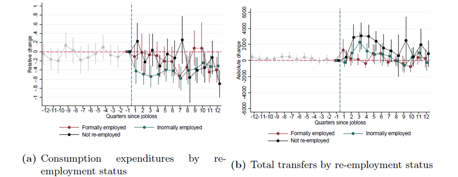
Figure A2. DID results on household transfers
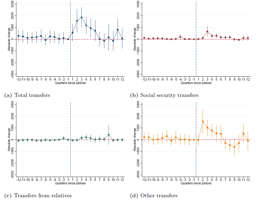
Figure A3. Results using an event study approach
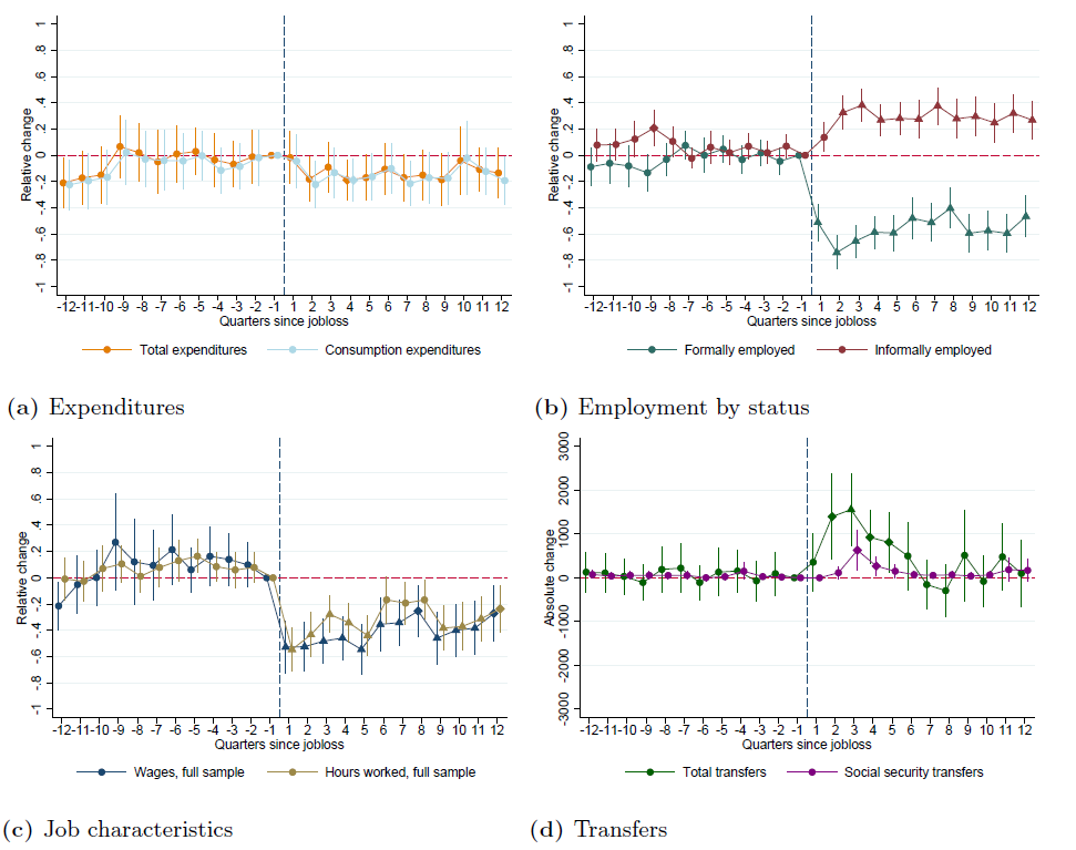
Figure A4. DID results without propensity score weights
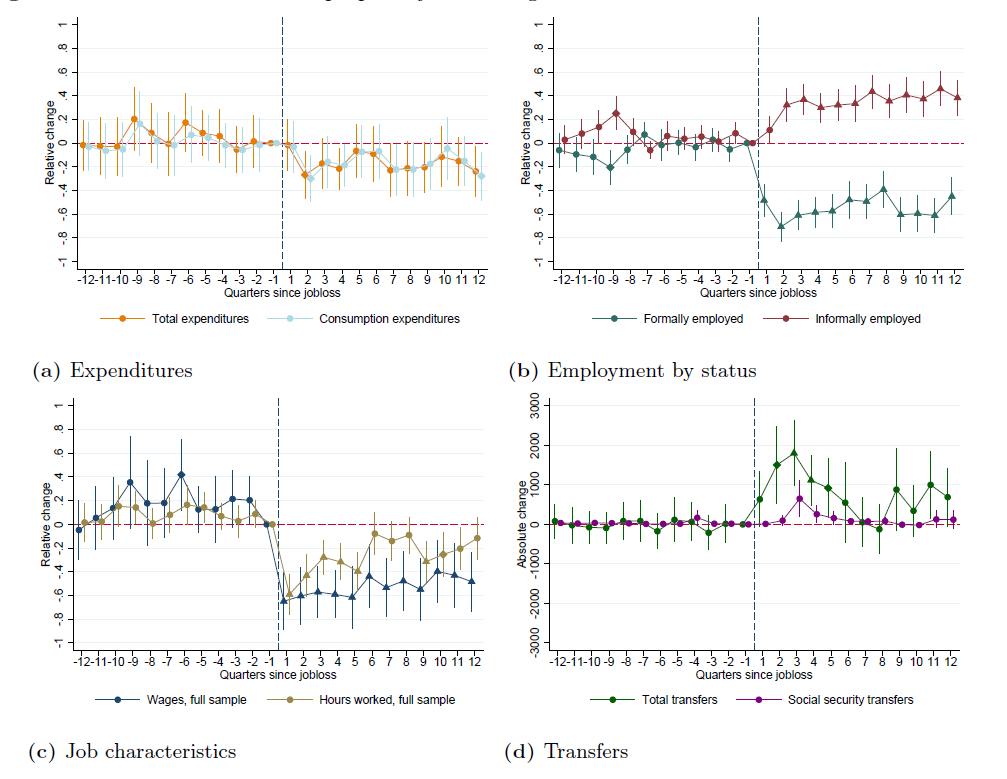
Figure A5. DID results on formal employment from panel and cross-sectional regressions
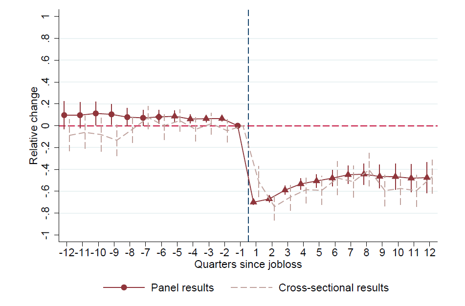
Figure A6. DID results on the sample of UB recipients dismissed for economic reasons
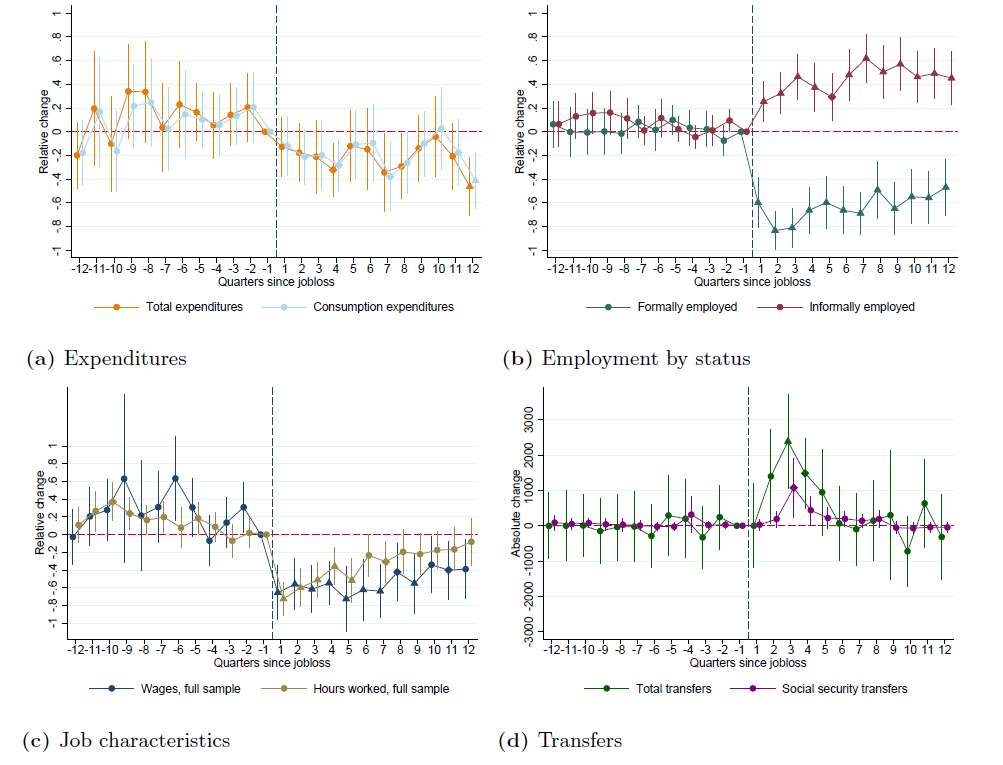
Figure A7. DID results on PES registration and work absenteeism
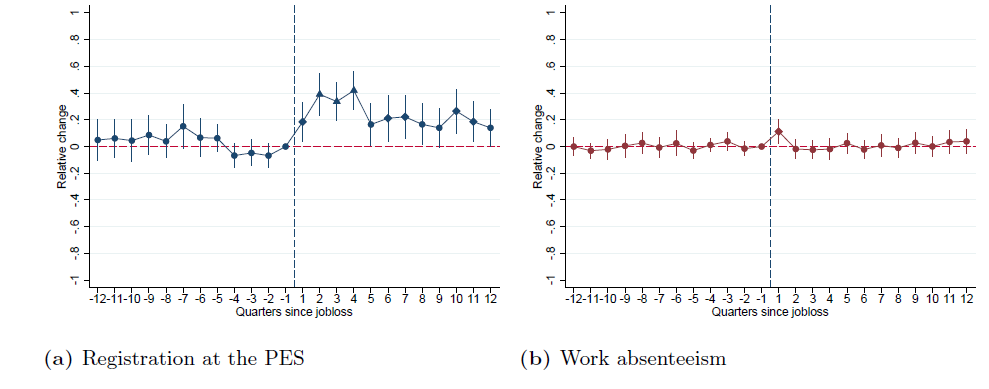
Figure A8. DID results on wages and total expenditures, by date of formal re-employment
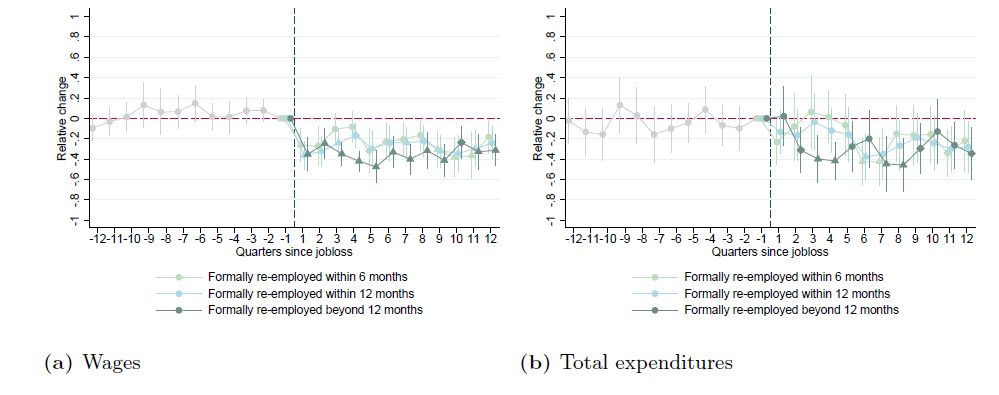
Figure A9. DID results on formal and informal wages, different specifications
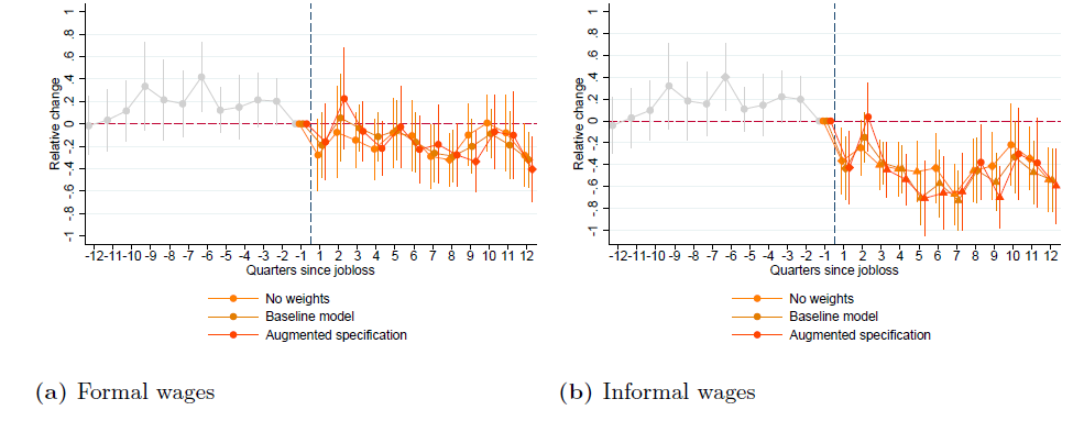
Figure A10. DID results on the sample of UB recipients around the upper bound
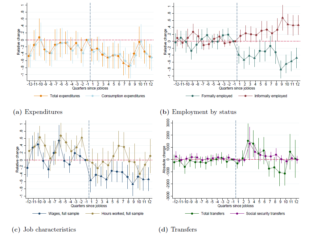
Table A1. Summary statistics for the DID analysis: treated and control groups
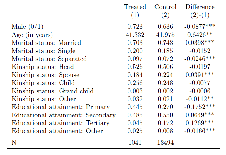
Appendix B: The efficiency costs of UBs and the substitution between formal and informal employment
Figure B1. Probability density function of the running variable around the lower bound
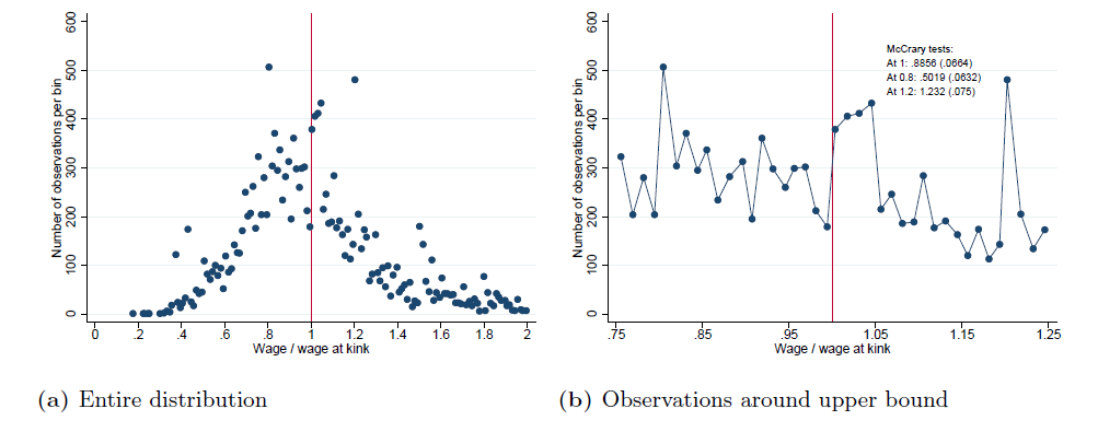
Figure B2. Evolution of covariates around the lower bound
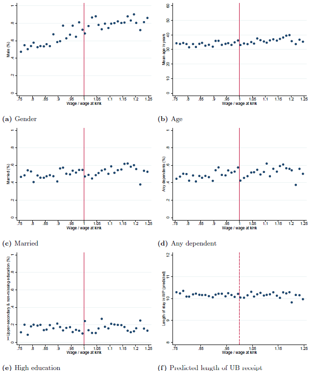
Figure B3. Scatter bin plot for the duration of UB receipt (in months) at the lower bound
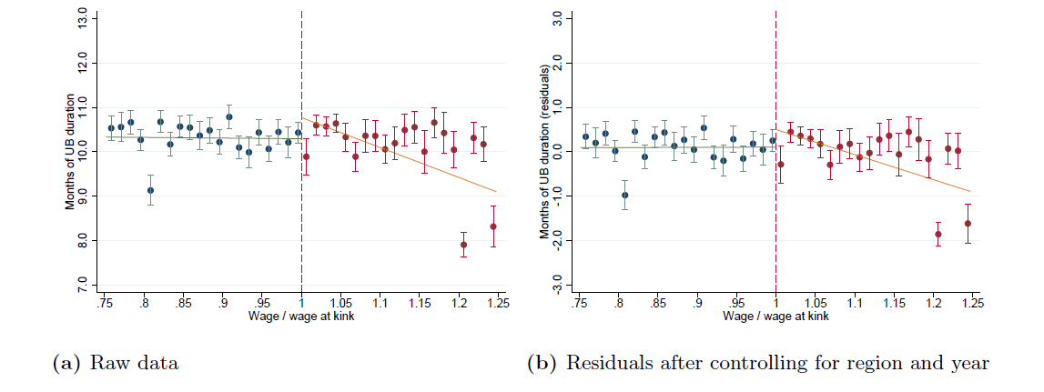
Figure B4. Scatter bin plots for formal and informal employment in selected months around job loss (upper bound)
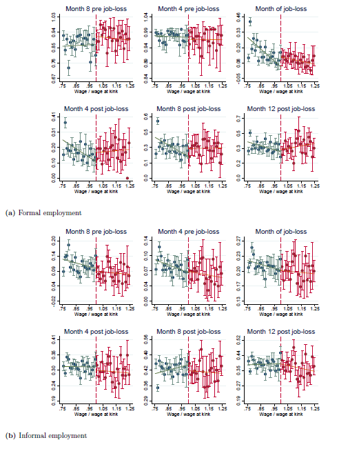
Figure B5. Scatter bin plot for the formal and informal employment in selected months around job loss (lower bound)
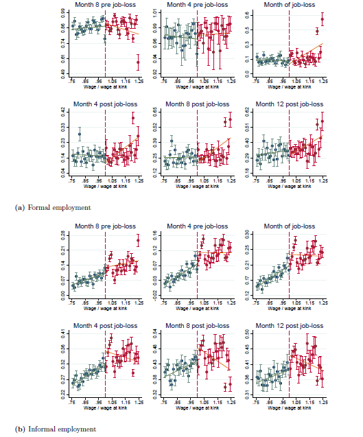
Figure B6. RK-results for the probabilities of being formally and informally employed in a given month around job loss, lower bound
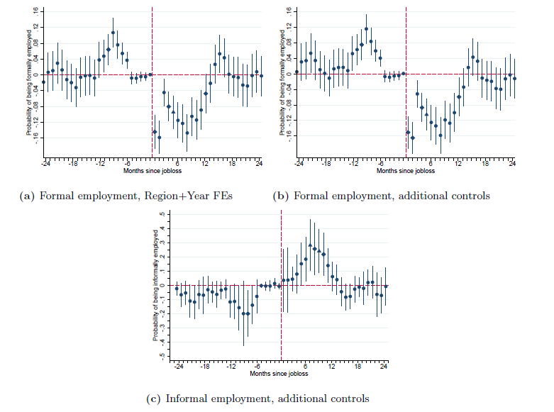
Figure B7. RK-results for the probabilities of being formally and informally employed in selected months after job loss, upper bound, by bandwidth
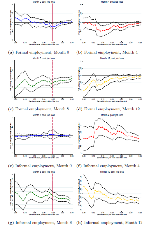
Figure B8. RK results for the duration of receiving UBs (months), upper bound, by bandwidth
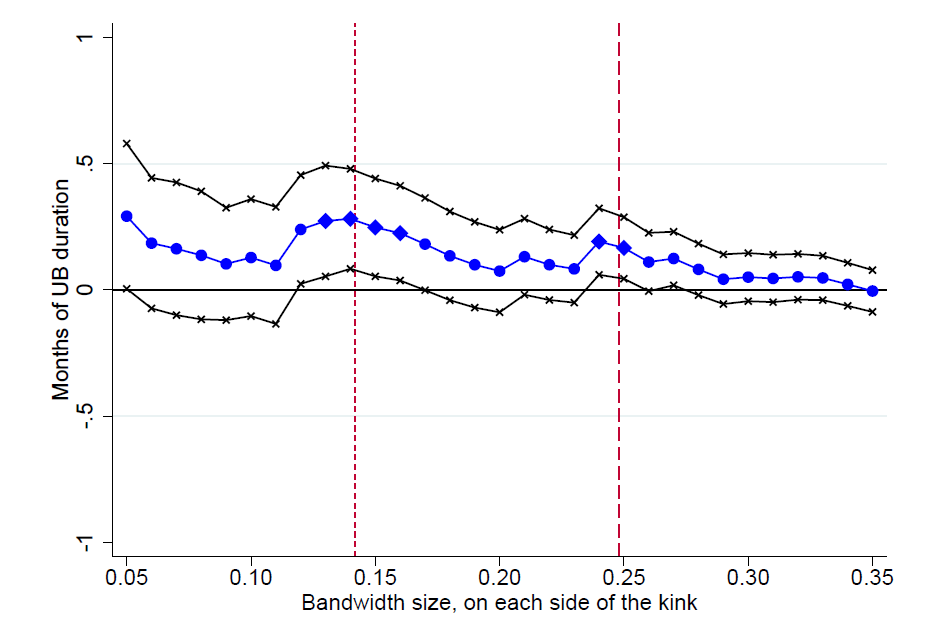
Figure B9. Detection of actual kink
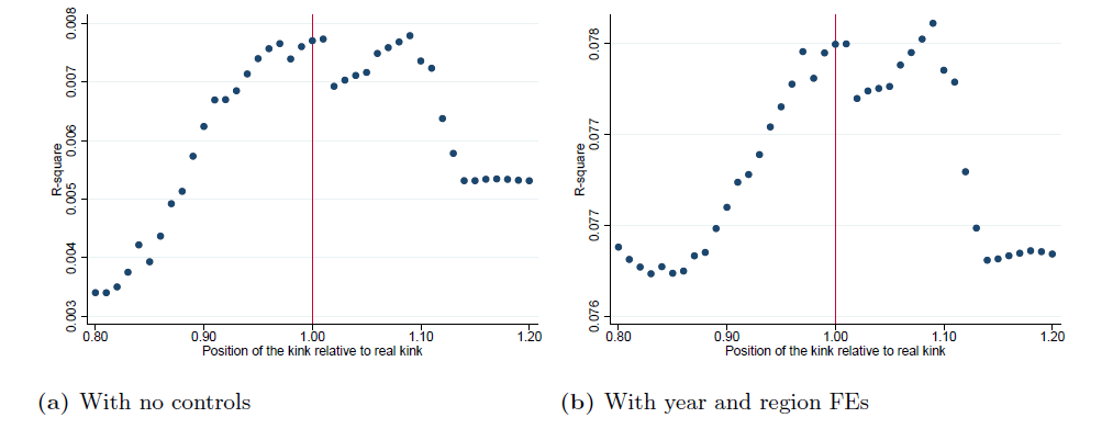
Table B1. Distribution of participants with UB entitlements at the lower and upper bounds, by year of participation and month of unemployment
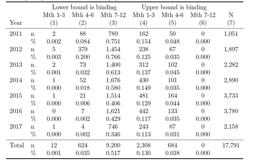
Table B2. Summary statistics for the RK analysis: overall sample and individuals in the proximity of the upper and lower bounds, respectively
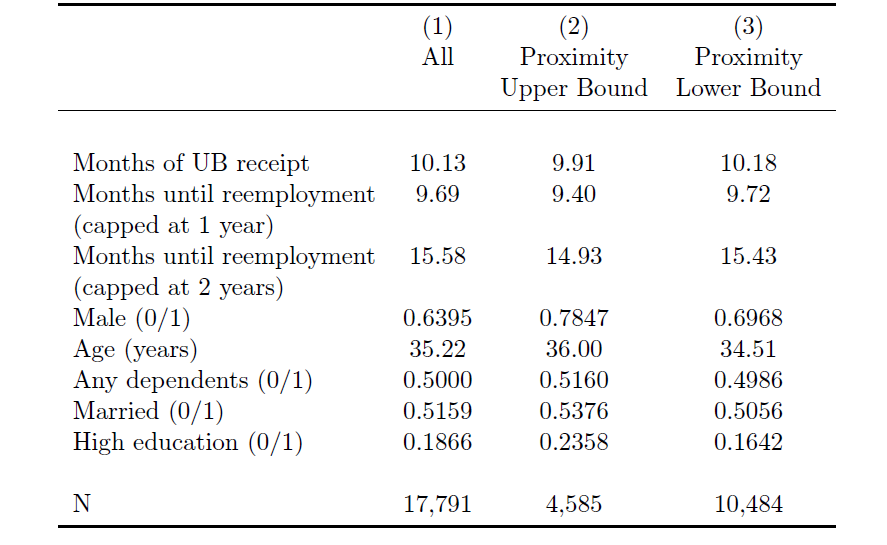
Table B3. Imputation regression for the likelihood of being informally employed in a given month around job loss
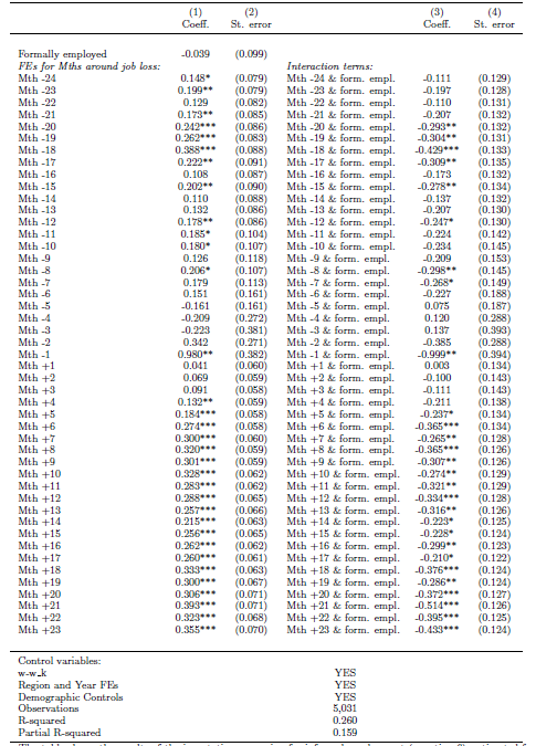
Table B4. Smoothness of covariates at the lower bound
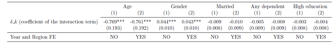
Table B5. RK-results for the duration of receiving UBs (months), lower bound
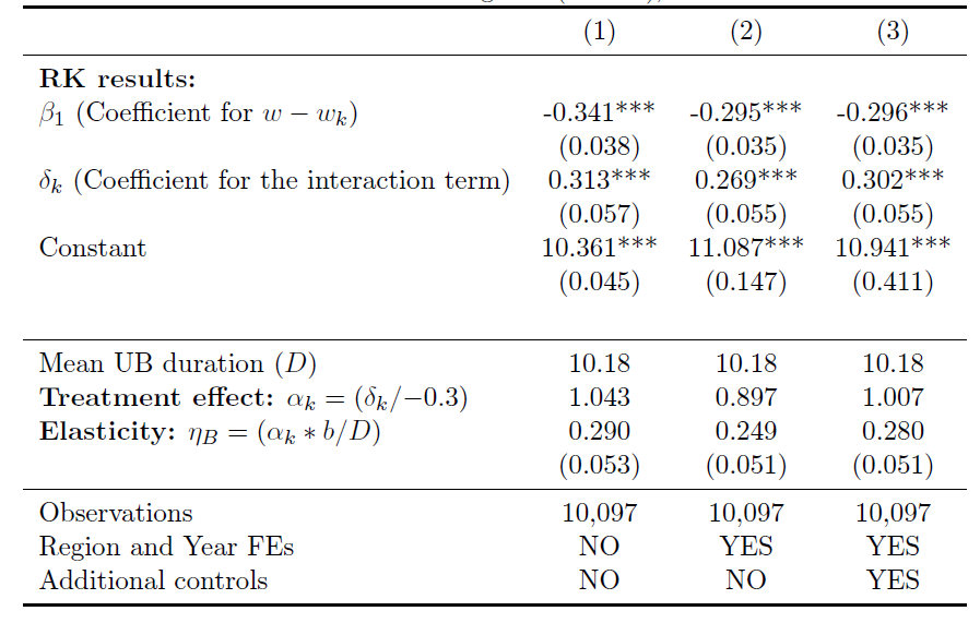
Table B6. Sensitivity of results to choice of the polynomial order, focusing on the probability of being formally employed in months 0, 4, 8, and 12 after job loss (upper bound)
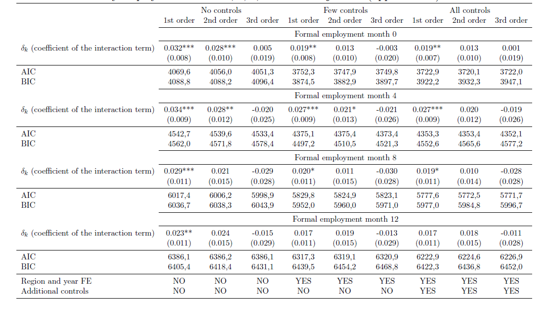
Table B7. Sensitivity of results to choice of the polynomial order, focusing on the imputed probability of being informally employed in months 0, 4, 8, and 12 after job loss (upper bound)
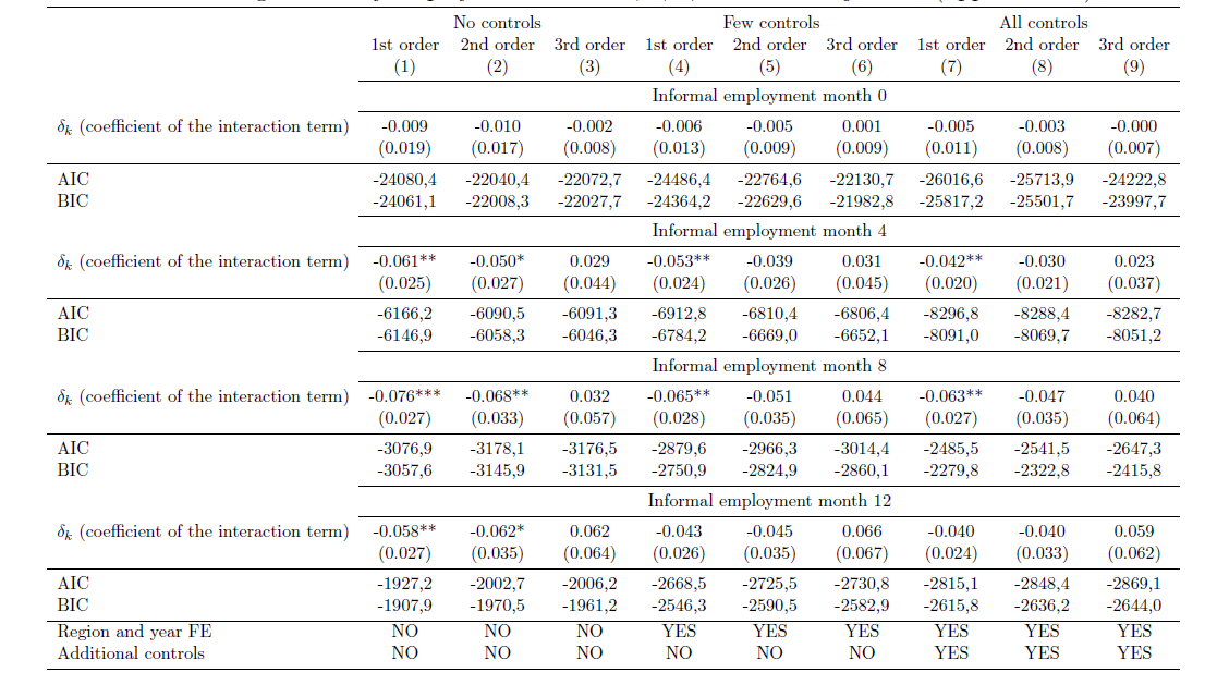
Table B8. Sensitivity of results to choice of the polynomial order, using the duration of receiving UBs (months) as the outcome variable (upper bound)
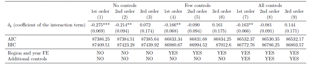
Table B9. RK-results for length of UB receipt using placebo running variable (upper bound)
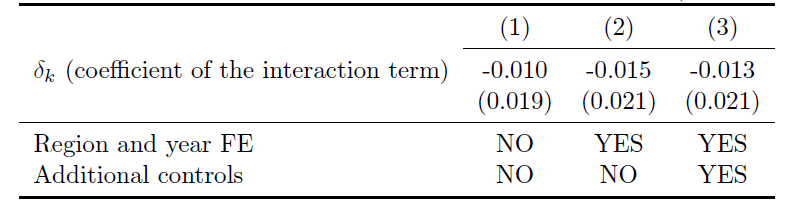
Table B10. Double difference RK-estimates (upper bound)