


Trade and Decent Work:
Adequate Earnings in the Mexican Manufacturing Industries
Abstract
This paper analyses the impact of non-preferential trade liberalization and exposure to globalization on “adequate earnings” in the Mexican manufacturing industries between 2003 and 2020, using data from the National Survey of Occupation and Employment and from the annual surveys of manufacturing industries. By means of panel data and three-stage least squares estimation strategies, it is found that, although exposure to globalization is not robustly associated with gross daily wages per employee, non-discriminatory trade liberalization and exposure to globalization contributed to a reduction in both the working poverty rate among employed persons and the share of employees with low pay rates. The paper is a contribution to the project “Trade, enterprises and labour markets: Diagnostic and firm level assessment (ASSESS)”, jointly funded by the European Commission and the ILO.
Introduction
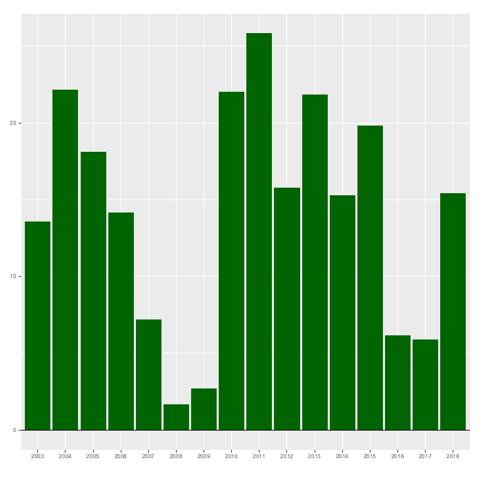
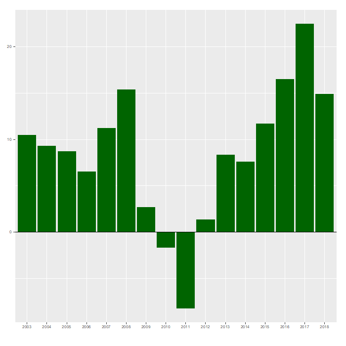
Over the past 15 years, the working poverty rate among employed persons – that is, the share of workers living in households whose per capita labour income is lower than the national poverty line – has increased considerably in Mexico (figure 1). Back in 2005, 31 per cent of the country’s labour force suffered working poverty. By 2020 this rate had increased by 9 percentage points (pp). Workers in the manufacturing sector have typically done better, exhibiting an average working poverty rate 6 pp lower than that in non-manufacturing sectors. This advantage, however, decreased by almost 13 per cent between 2005 and 2020 (figure 2). A very similar pattern is observed in the share of employees with low pay rates, that is, the fraction of workers who are paid less than two-thirds of median earnings in the labour market (figures 3 and 4). The International Labour Organization (ILO) has proposed that the working poverty rate among employed persons and the share of employees with low pay rates are the main statistical indicators by which countries can monitor their progress in delivering “adequate earnings”, understood as “a just share of the fruits of progress to all, and a minimum living wage to all employed” (ILO 2013, 65). Adequate earnings are one of the ten substantive elements of the Decent Work Agenda.1
During the same period, Mexico deepened the trade liberalization and globalization processes that began in 1986 when the country joined the General Agreement on Tariffs and Trade (GATT). It subscribed to seven new trade agreements,2 making a total of 13 with 50 countries; to 17 new agreements on the promotion and reciprocal protection of investment, making a total of 32 with 33 countries; and to three new economic complementation and partial scope agreements within the framework of the Latin American Integration Association (ALADI), making a total of nine (Secretaría de Economía 2016). Although the most significant trade events for the Mexican economy – such as the GATT accession and the North American Free Trade Agreement (NAFTA) (replaced in July 2020 with the United States–Mexico–Canada Agreement – USMCA) – occurred in the last two decades of the twentieth century,3 this continued integration effort in the early years of the new millennium translated into a further 11 pp reduction in the country’s trade-weighted average non-preferential import tariff (figure 5) and a 27 pp increase in its level of trade openness as measured by the ratio of the sum of imports and exports to the GDP (figure 6).
In the light of all this, it may be tempting to jump to the conclusion that perhaps trade liberalization and globalization have had a prejudicial role in the rise of working poverty and relatively low wages in Mexico, since these two measures of adequate earnings are negatively correlated with the level of import tariffs and positively correlated with trade openness (figure 7). But the data also indicate that the tradable and highly globalized sector of manufacturing has not strongly diverged from other economic sectors and that the manufacturing industries’ greater exposure to globalization (measured by the shares of imported inputs in total inputs and of exports in total sales) is not clearly associated with lower wages (figure 8). On top of this, it is worth keeping in mind that some of the trade agreements recently signed by Mexico include labour provisions that set framework conditions for decent work (Sánchez Gómez et al. 2021).
So, how do trade liberalization and exposure to globalization relate to adequate earnings? The theory and empirical evidence on trade and its implications for labour markets and decent work are quite extensive (Aleman-Castilla 2020), but much of the attention has focused on a small group of outcomes, such as wages (e.g., Helpman et al. 2017; Lee and Lee 2015; Krishna, Poole and Senses 2014; Kovak 2013), employment (e.g., Dix-Carneiro and Kovak 2017; Coşar, Guner and Tybout 2016; Autor, Dorn and Hanson 2013) or informality (e.g., Dix-Carneiro et al. 2021; Ben Salem and Zaki 2019; Ulyssea and Ponczek 2018; Cruces, Porto and Viollaz 2018). Although the study of other aspects has expanded recently (e.g., Ben Yahmed 2017, Hakobyan and McLaren 2017 and Juhn, Gergely and Villegas-Sanchez 2014 on gender disparities; or Kis-Katos and Sparrow 2011, Edmonds, Pavcnik and Topalova 2010 and Olarreaga, Saiovici and Ugarte 2020 on child labour), the evidence regarding working poverty – which relates not only to wages and employment opportunities but also to household size and national poverty lines – is still relatively scarce and ambiguous (ILO 2021). In theory, trade openness should help to reduce poverty (Bhagwati and Srinivasan 2002; Ohlin 1933), but cross-country empirical studies have found that this effect depends on country-specific factors such as trade policies, labour market institutions or even transport infrastructure (Mitra 2016), and that it varies significantly across economic sectors and between rural and urban areas (World Bank Group and WTO 2018 and 2015).
To date, most of the single-country studies have used data from one side of the labour market only, typically from labour force surveys, national censuses or administrative sources. Only recently have researchers begun to make more frequent use of linked employer–employee datasets (LEEDs) (e.g., Dix-Carneiro and Kovak 2019; Alfaro-Urena, Manelici and Vásquez 2019; Schröder 2018). This type of data allows researchers to control for firms’ and workers’ heterogeneity and for characteristics specific to the employment relationship (Mittag 2019; Woodcock 2015; Bryson, Forth and Barber 2006). LEEDs are particularly useful in studying the wage structures of firms, employment mobility, and race and gender discrimination (Abowd, Kramarz and Woodcock 2008). But, despite these advantages, the collection of LEEDs is often expensive and complicated, which partly explains why they have not been more widely used (Jensen 2010).
An alternative could be the complementary use of labour force and establishment surveys.4 Whereas the former tend to have little information about workplaces, the latter typically provide scarce data about workers (ILO 2020). However, it is usually possible to link the two at a certain level of aggregation, after separately controlling for worker and establishment characteristics. This paper does precisely that in order to study the effects of non-preferential trade liberalization (i.e., the reduction of the industry-average Most Favoured Nation (MFN) import and export tariffs) and exposure to globalization (i.e., the extent to which domestic firms rely on foreign inputs and markets for the production and sales of finished goods) on adequate earnings in the Mexican manufacturing sector between 2003 and 2020. It provides new evidence on the impact of trade on working poverty, using alternative measures that go beyond those traditionally analysed in studies in this field. Two complementary econometric estimation strategies are used for this purpose. First, a panel data procedure applied to firm-level data from the 2003–09 Annual Industrial Survey (EIA-03) and the 2009–18 Annual Manufacturing Industry Surveys (EAIM-09 and EAIM-13) is used to look at the relationship between gross daily wages per employee and exposure to globalization. Second, a three-stage least squares estimation approach is used to link these surveys with the 2005–20 National Survey of Occupation and Employment (ENOE) at the four-digit industry level of the North American Industry Classification System (NAICS), and with the 2003–17 trade data available from the World Trade Organization’s (WTO’s) DATA and Tariff Download Facility, to estimate the effect of non-preferential trade liberalization and exposure to globalization on the working poverty rate among employed persons and the share of employees with low pay rates.
The main results can be deemed consistent with the theories of trade where there is firm heterogeneity (e.g., Sampson 2014; Yeaple 2005; Melitz 2003) and with previous findings from related empirical studies (e.g., Matthee, Rankin and Bezuidenhout 2017; Verhoogen 2008; Schank, Schnabel and Wagner 2007). In the manufacturing sector, although gross daily wages per employee were higher in more productive firms and in those with larger shares of income from maquila, sub-maquila and re-manufacture services,5 they were not affected by exposure to globalization. On the other hand, non-preferential trade liberalization and higher exposure to globalization contributed to a reduction in both the working poverty rate among employed persons and the share of employees with low pay rates and to a widening of the differences in these two indicators between formal and informal workers. The rest of the paper is organized as follows. Section 1 describes the data and decent work indicators used and presents a preliminary statistical analysis of their distributions and their relationships with the globalization and trade liberalization variables. Section 2 explains the econometric approaches and presents the corresponding results. The last section concludes.
Data and preliminary analysis
This study focuses on the impact of non-preferential
-
Gross daily wages per employee (GDWE or
wages ) – an establishment-level variable equal to the average gross wage and benefits6 paid per working day to each worker directly employed by the firm in core production activities. -
Working poverty rate of employed persons (WPRE or
working poverty ) – an individual-level indicator for workers aged 15 or over, which is equal to 1 if the person lives in a household whose total monthly income is below the national poverty line7 and is equal to 0 otherwise. -
Employees with low pay rates (ELPR or
low-wage workers ) – an individual-level indicator for occupied workers aged 15 or over, which is equal to 1 if the person is paid less than two-thirds of the median earnings in the labour market and is equal to 0 otherwise.
1.1 Firm, worker and trade data
Given that the objective is to assess the impact of trade on adequate earnings after controlling for worker and firm characteristics, data from the following surveys by the Mexican National Institute for Statistics and Geography (INEGI) are used: the 2003–08 Annual Industrial Survey (EIA-03); the 2009–18 Annual Survey of the Manufacturing Industry (EAIM-09 and EAIM-13); and the 2005–18 first quarters of the National Survey of Occupation and Employment (ENOE). The EIA and EAIM are annual panel-structured surveys that follow manufacturing establishments over time, classifying them into industries according to the six-digit level of the NAICS, and collecting annual information about their labour force; remuneration; hours and days worked; costs, revenues and value of production; inventories; and fixed assets. The EIA-03 covered 231 industries under the 2002 NAICS, followed 7,294 establishments and excluded export-oriented maquiladoras. The EAIM-09 replaced the EIA-03, adding nine more industries under the 2007 NAICS, increasing the number of establishments to 11,455 and including export-oriented maquiladoras. In 2017 INEGI generated the new series EAIM-13, adjusting the number of establishments in the sample to 10,447 and the industries covered to 239 under the 2013 NAICS.8 The design of these surveys was based on the International Recommendations for Industrial Statistics of the United Nations
The ENOE, on the other hand, is the quarterly rotating-panel national labour market survey available since 2005. Following households and individuals for five consecutive trimesters, this survey collects data on sociodemographic characteristics such as kinship, sex, age, education, marital status, number of children and geographic location; as well as labour market characteristics for the working-age population (15 years and older), such as economic activity status, occupation, economic sector, size and location of employer, wages, working time, social security coverage and unemployment spells, among others. Since their origin more than 45 years ago, the Mexican labour market surveys have used the ILO criteria as their basic conceptual reference. However, to ensure comparability with new recommendations and to raise information quality standards, they have also considered the conceptual frameworks of other international bodies such as the Organization of Economic Cooperation and Development (OECD) and the United Nations Statistics Division
Finally, data from the WTO are used to obtain measures of trade liberalization. Among other topics, the WTO’s DATA and Tariff Download Facility11 provide information on MFN applied and bound tariffs, bilateral imports, market access conditions facing exports in top-five export markets, and non-tariff measures indicators for all WTO Members registered under the standard Harmonized System (HS). The MFN tariffs are the normal non-discriminatory duties that a WTO Member charges on imports that are excluded from any free trade or preferential agreement. In this sense, they represent an upper limit for actual trade taxes, since they apply between countries that do not have an agreement, or to products that do not comply with the rules of origin agreed in an agreement. Given that in the period of interest Mexico signed seven new trade deals, which all entered into force at different times, and that this study is interested in the country’s aggregate non-preferential trade liberalization experience, the MFN applied tariffs are a suitable indicator to employ. Besides being an adequate measure of applicable trade duties for the period before each free trade agreement entered into force, and an upper limit thereafter, MFN tariffs are still binding for some important trade relationships, such as the one with China, which is Mexico’s fourth-largest trade partner.12 Figure 5 shows the trade-weighted averages of the ad valorem equivalent (AVE) MFN tariffs applied on Mexican imports (TWAIT or
1.2 Preliminary analysis
This subsection presents a first glance at the distribution characteristics of
Figures 12 to 14 show the boxplots for these means now grouped by year. There is no clear time trend for
Moving now to the ENOE data, figures 17 and 18 present the boxplots for the four-digit NAICS annual means of
This preliminary analysis yields some interesting insights. First, from the establishment-level data, the gross daily wages per employee, the share of imported inputs in total inputs, and the share of exports in total sales all have high variability across industries, suggesting that group effects are important. Second, changes in gross daily wages seem to be positively correlated with changes in the share of imported inputs and negatively correlated with changes in the share of exports. Third, from the worker-level data, the working poverty rate among employed persons and the share of employees with low pay rates also have important variability across sectors, among which manufacturing registers close to the average. And, fourth, there seems to be a positive correlation between changes in these two decent work indicators and changes in the trade liberalization variables, implying that lower non-preferential import and export tariffs will be associated with more adequate earnings across tradable industries.
Econometric analysis
As described above, the econometric analysis consists of two parts. First, a panel data estimation procedure is carried out on pooled data from the EIA-03, EAIM-09 and EAIM-13 establishment surveys, to look at the relationship between
2.1 Panel data
The effect of exposure to globalization on
(1)
where is the natural logarithm of
2.2 Three-stage least squares
The effect of trade liberalization and exposure to globalization on
(2)
where refers to each of the
(3)
where is a dummy variable for informal workers, and and are matrices of interactions of the vector and the industry dummies, respectively, with this informality indicator. The coefficients capture the variation that is attributable to differences in individual characteristics between formal and informal workers, and the coefficients capture the variation that is attributable to differences in industry affiliation. In the second stage, a linear model is estimated using the EIA and EAIM establishment surveys’ data, for each year in the samples:
(4)
where refers to each of the two variables of exposure to globalization
(5)
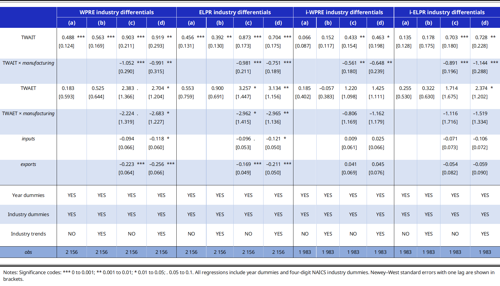
where refers to each of the industry differentials and , is the vector of
A. First stage results
Estimation of the parameters in equations (2) and (3) is useful to study the determinants of
B. Second stage results
As with the worker-level data, the estimation of the parameters in equation (4) can be used to analyse the relationship between the establishment characteristics and the level of exposure to globalization. The corresponding results are reported in tables 8 and 9. For most years in the sample, the share of
C. Third stage results
After controlling for worker and establishment characteristics, the third and last step consists of estimating the parameters of equation (5). Table 10 reports the corresponding results. For each dependent variable, column (a) presents the estimates obtained when only the
In sum, the first stage of the analysis demonstrates that
Conclusions
This paper has investigated the effect of non-preferential trade liberalization and exposure to globalization on adequate earnings in Mexican manufacturing industries between 2003 and 2020. During this period, when the country subscribed to seven new trade agreements, 17 new bilateral investment agreements and three new economic complementation agreements, the proportion of its people experiencing working poverty and low wages increase by 9 and 4 pp, respectively. Although it may be tempting to infer that non-discriminatory trade liberalization and a higher exposure to globalization have had a prejudicial role, the analysis suggests that they have not. Panel data estimations using the 2003–18 surveys of manufacturing establishments indicate that, although gross daily wages per employee are higher in more productive firms, and in those with larger shares of income from maquila, sub-maquila and re-manufacture services, they are not significantly related to the share of imported inputs in total inputs or to the share of exports in total net sales. Using a three-stage least squares procedure, these establishment surveys were linked to the 2005–20 national labour force survey and to MFN tariff and trade data from the WTO. After controlling separately for observable characteristics of establishments and workers, it was found that recent non-preferential trade liberalization and higher exposure to globalization contributed in Mexican manufacturing industries to a reduction in working poverty and the share of employees with low pay rates. However, MFN trade liberalization also contributed to an expanding gap in adequate earnings between formal and informal workers.
Annex
Figure 1. Working poverty rate of employed persons (WPRE) (percentage of employed persons living in households with incomes below the national poverty line)
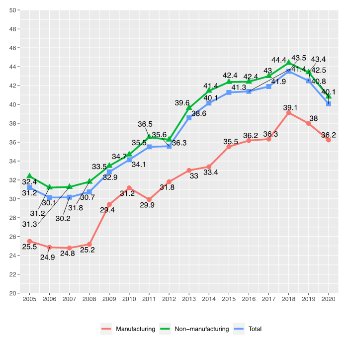
Source: Author’s calculations using labour force data from ENOE (INEGI) and the national urban poverty lines (CONEVAL).
Figure 2. WPRE gap between manufacturing and non-manufacturing industries (ratio of WPRE manufacturing to WPRE non-manufacturing)
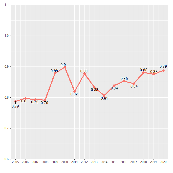
Source: Author’s calculations using labour force data from ENOE (INEGI) and the national urban poverty lines (CONEVAL).
Figure 3. Employees with low pay rates (ELPR) (percentage of employees paid less than two-thirds of median earnings)
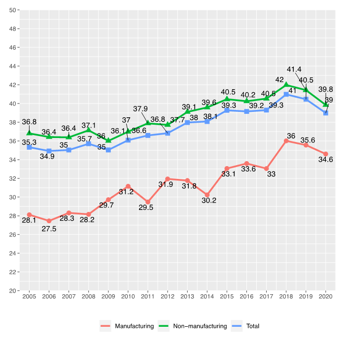
Source: Author’s calculations using labour force data from ENOE (INEGI).
Figure 4. ELPR gap between manufacturing and non-manufacturing industries (ratio of ELPR manufacturing to ELPR non-manufacturing)
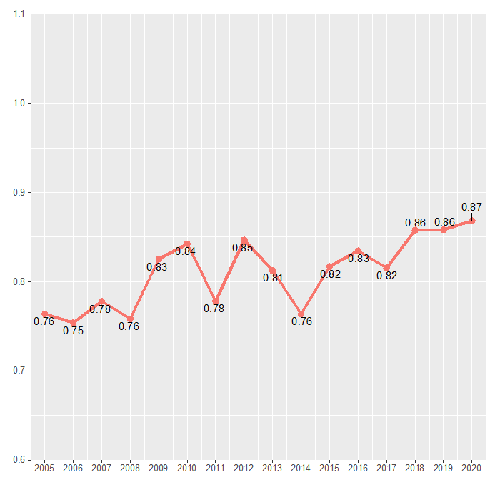
Source: Author’s calculations using labour force data from ENOE (INEGI).
Figure 5. Weighted average tariffs on Mexican imports and exports, 2003–17
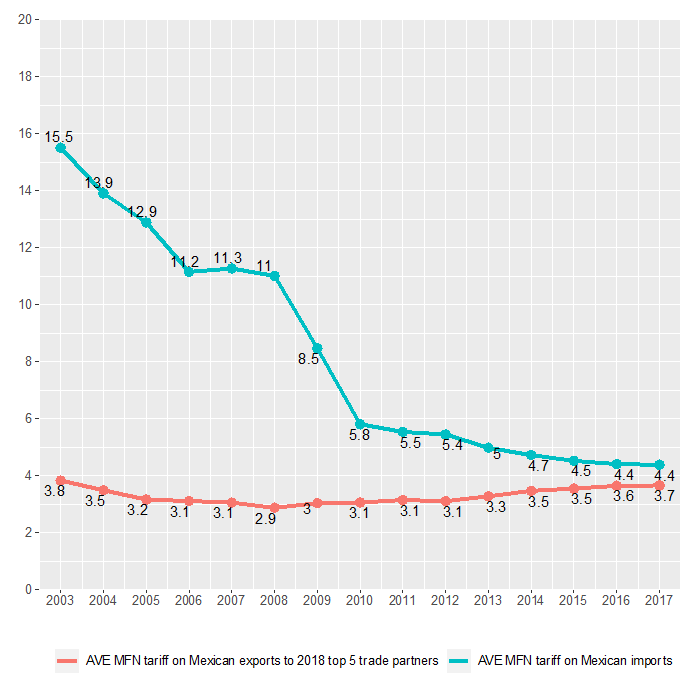
Note: Weights equal to import/export volumes at the six-digit HS level.
Source: Author’s calculations with data from WTO.
Figure 6. Trade openness in Mexico, 1950–2017
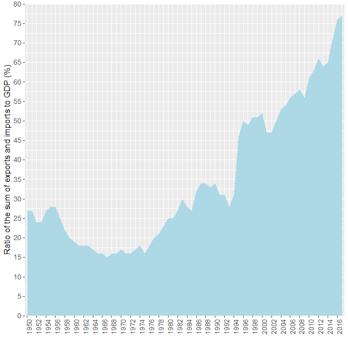
Source: Our World in Data. Trade Openness, 1950 to 2017, Oxford Martin School, University of Oxford
(available at https://ourworldindata.org/trade-and-globalization), based on work by Feenstra, Inklaar and Timmer (2015).
Figure 7. Correlations for trade and decent work indicators
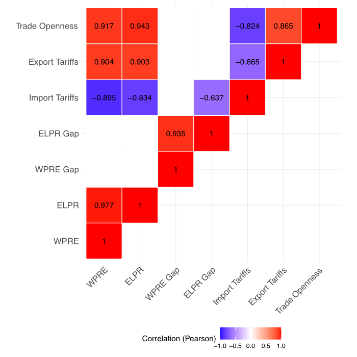
Notes: Trade Openness = sum of imports and exports as percentage of GDP; Import Tariffs = weighted average MFN import
tariff; Export Tariffs = weighted average MFN export tariffs to top five partners; WPRE = working poverty rate of employed
persons; ELPR = employees with low pay rates; WPRE Gap = WPRE manufacturing / WPRE non-manufacturing; ELPR Gap = ELPR
manufacturing / ELPR non-manufacturing. Only significant correlations (at a 5 per cent level) are shown.
Source: Author’s calculations using data from ENOE (INEGI), WTO and Our World in Data (based on Feenstra, Inklaar and
Timmer 2015).
Figure 8. Globalization and gross daily wages per employee (GDWE) (2003–18 weighted average figures for three-digit NAICS Mexican manufacturing)
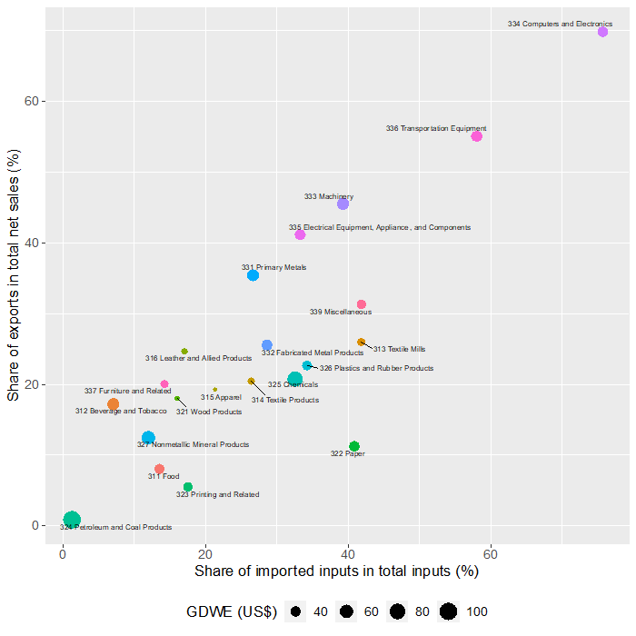
Note: Weights equal to the number of establishments surveyed for each year-subsector.
Source: Author’s calculations using data from the establishment-level surveys for the manufacturing sector EIA-03, EAIM-09 and EAIM-13 (INEGI).
Figure 9. Gross daily wages per employee (GDWE) (distribution of four-digit NAICS annual means, grouped by three-digit NAICS subsector)
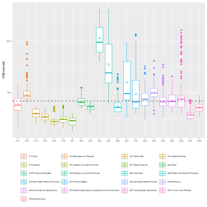
Note: Triangles represent weighted means for each three-digit NAICS subsector. The dashed line indicates the weighted mean for the full sample.
Figure 10. Share of imported inputs in total inputs (
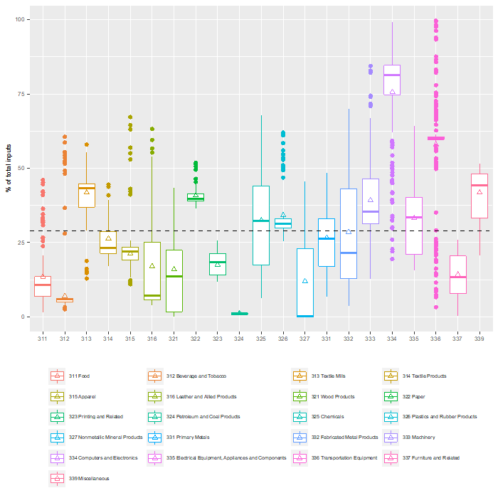
Note: Triangles represent weighted means for each three-digit NAICS subsector. The dashed line indicates the weighted mean for the full sample.
Figure 11. Share of exports in total sales (
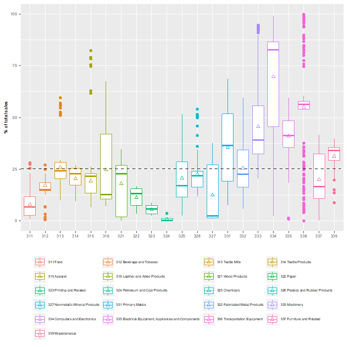
Note: Triangles represent weighted means for each three-digit NAICS subsector. The dashed line indicates the weighted mean for the full sample.
Figure 12. Gross daily wages per employee (GDWE) (distribution of four-digit NAICS means for each year in the sample)
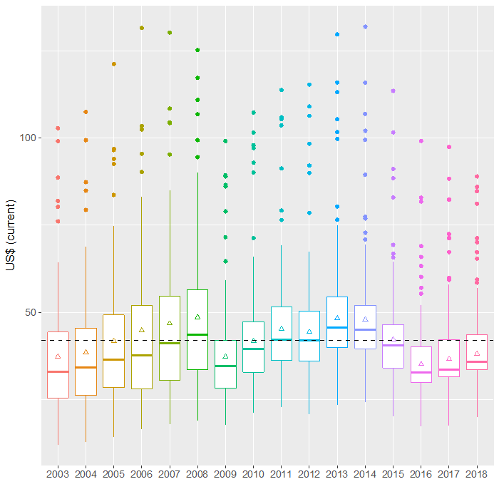
Note: Triangles represent weighted means for each year. The dashed line indicates the weighted mean for the full sample.
Figure 13. Share of imported inputs in total inputs (
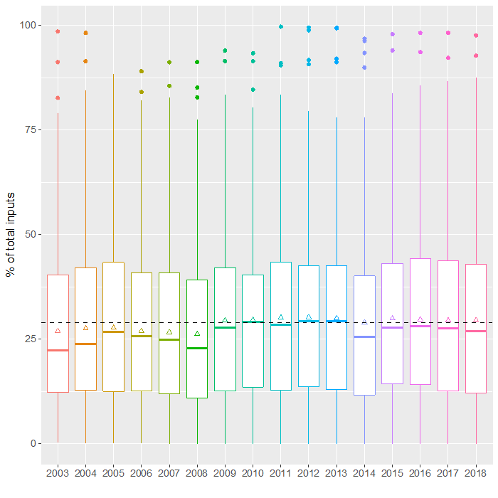
Note: Triangles represent weighted means for each year. The dashed line indicates the weighted mean for the full sample.
Figure 14. Share of exports in total sales (
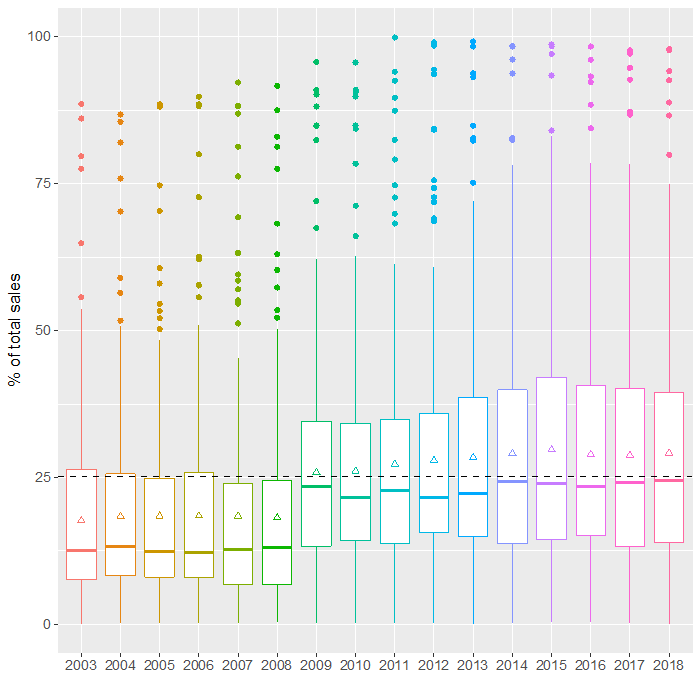
Note: Triangles represent weighted means for each year. The dashed line indicates the weighted mean for the full sample.
Figure 15. Share of imported inputs (
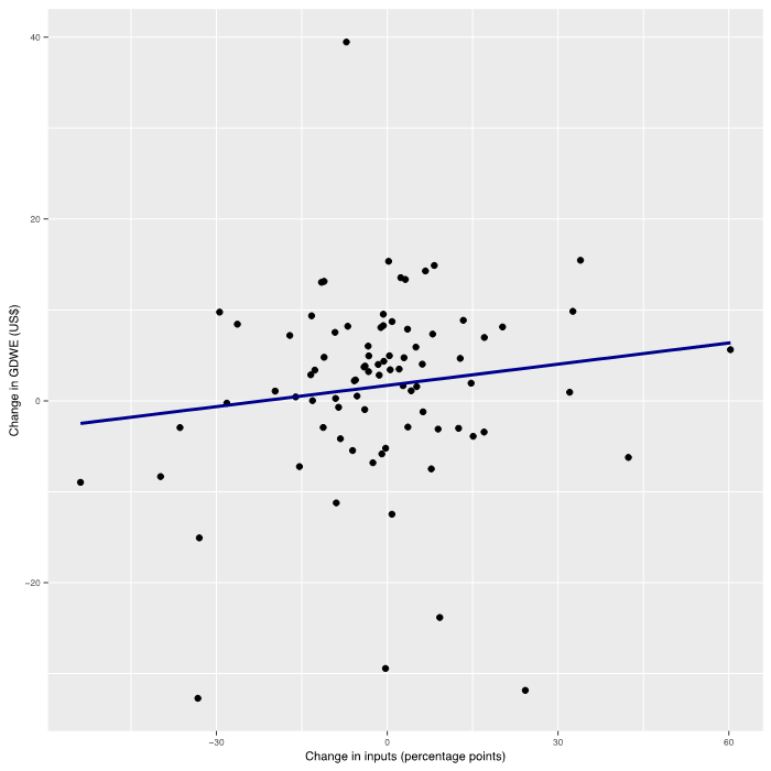
Note: Observations are four-digit NAICS industry mean values. The estimated equation of the simple regression line is .
Figure 16. Share of exports (
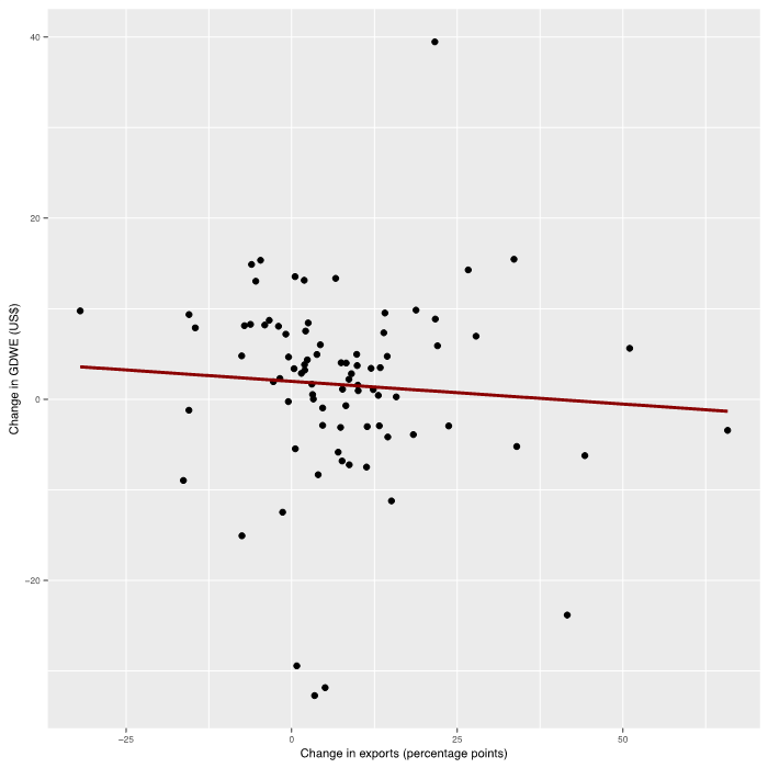
Note: Observations are four-digit NAICS industry mean values. The estimated equation of the simple regression line is .
Figure 17. Working poverty rate of employed persons (WPRE) (distribution of four-digit NAICS annual means, grouped by two-digit NAICS sectors)
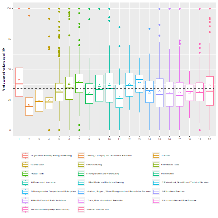
Note: Triangles represent weighted means for each two-digit NAICS sector. The dashed line indicates the weighted mean for the full sample.
Figure 18. Employees with low pay rates (ELPR) (distribution of four-digit NAICS annual means, grouped by two-digit NAICS sectors)
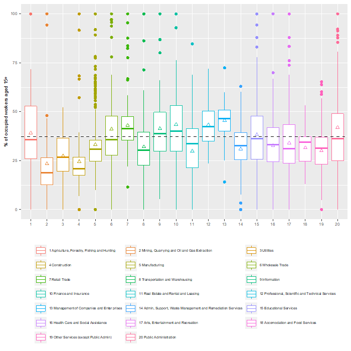
Note: Triangles represent weighted means for each two-digit NAICS sector. The dashed line indicates the weighted mean for the full sample.
Figure 19. Working poverty rate of employed persons (WPRE) (distribution of four-digit NAICS means for each year in the sample)
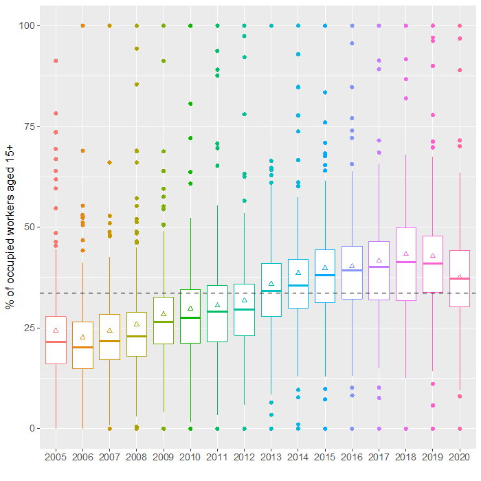
Note: Triangles represent weighted means for each year. The dashed line indicates the weighted mean for the full sample.
Figure 20. Employees with low pay rates (ELPR) (distribution of four-digit NAICS means for each year in the sample)
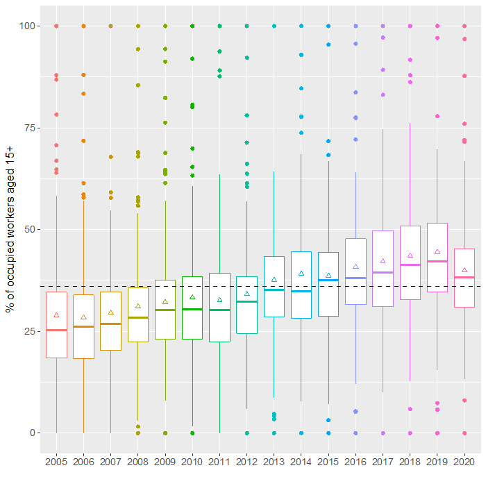
Note: Triangles represent weighted means for each year. The dashed line indicates the weighted mean for the full sample.
Figure 21. Trade-weighted average import tariffs (TWAIT) vs. working poverty rate of employed persons (WPRE), 2005–17
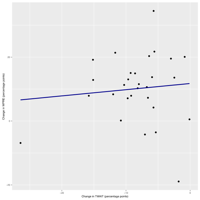
Note: Observations are four-digit NAICS mean values for tradable industries only. The estimated equation of the simple
regression line is .
Figure 22. Trade-weighted average export tariffs (TWAET) vs. working poverty rate of employed persons (WPRE), 2005–17
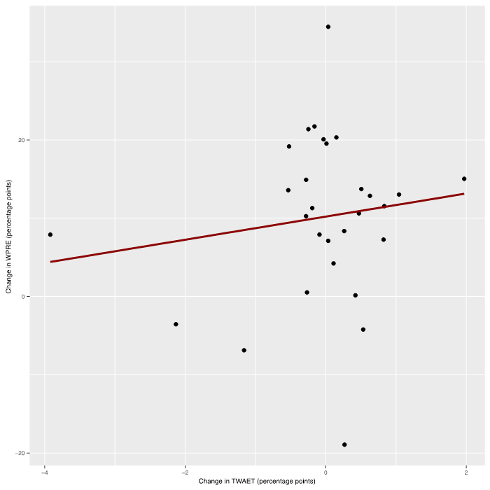
Note: Observations are four-digit NAICS mean values for tradable industries only. The estimated equation of the simple
regression line is .
Figure 23. Trade-weighted average import tariffs (TWAIT) vs. employees with low pay rate (ELPR), 2005–2017
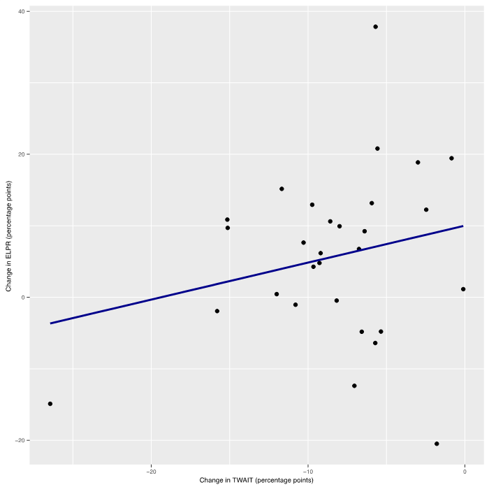
Note: Observations are four-digit NAICS mean values for tradable industries only. The estimated equation of the simple
regression line is .
Figure 24. Trade-weighted average export tariffs (TWAET) vs. employees with low pay rate (ELPR) 2005–2017
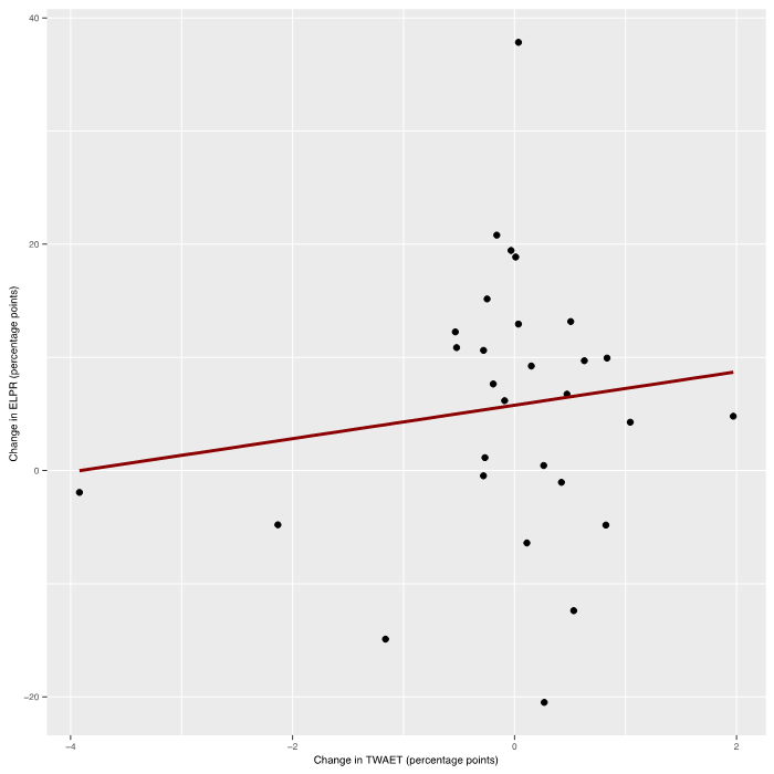
Note: Observations are four-digit NAICS mean values for tradable industries only. The estimated equation of the simple
regression line is .
Figure 25. Working poverty rate for employed persons (WPRE) (weighted average differentials for manufacturing and non-manufacturing industries, four-digit NAICS level)
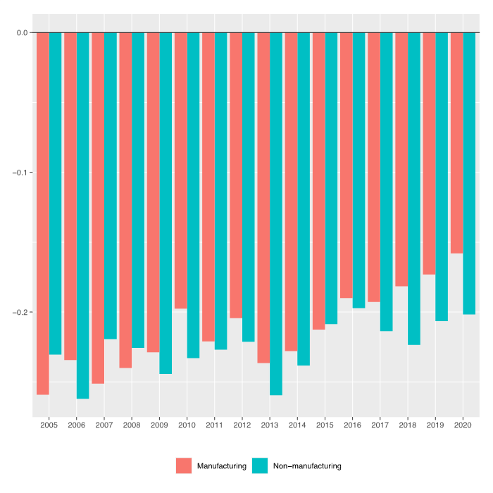
Note: Weights are equal to the inverse of the variance of the corresponding estimated coefficients.
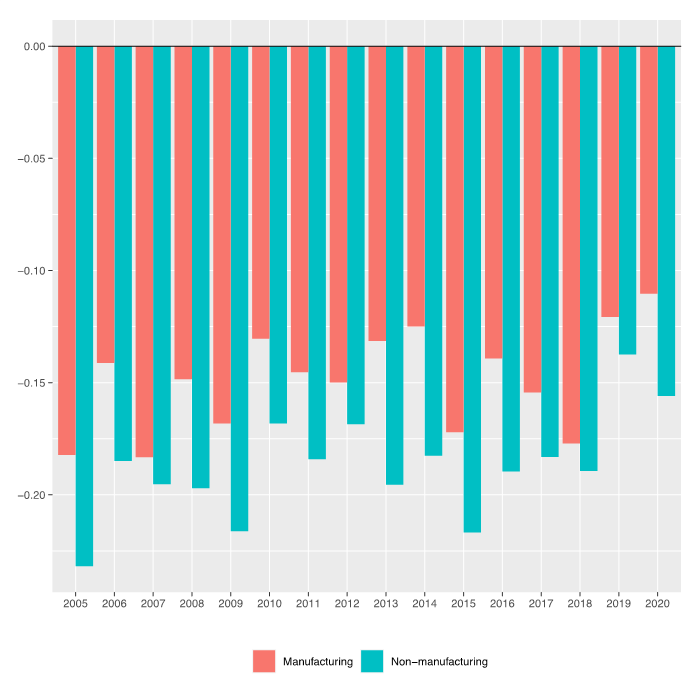
Figure 26. Employees with low pay rates (ELPR) (weighted average differentials for manufacturing and non-manufacturing industries, four-digit NAICS level)
Note: Weights are equal to the inverse of the variance of the corresponding estimated coefficients.
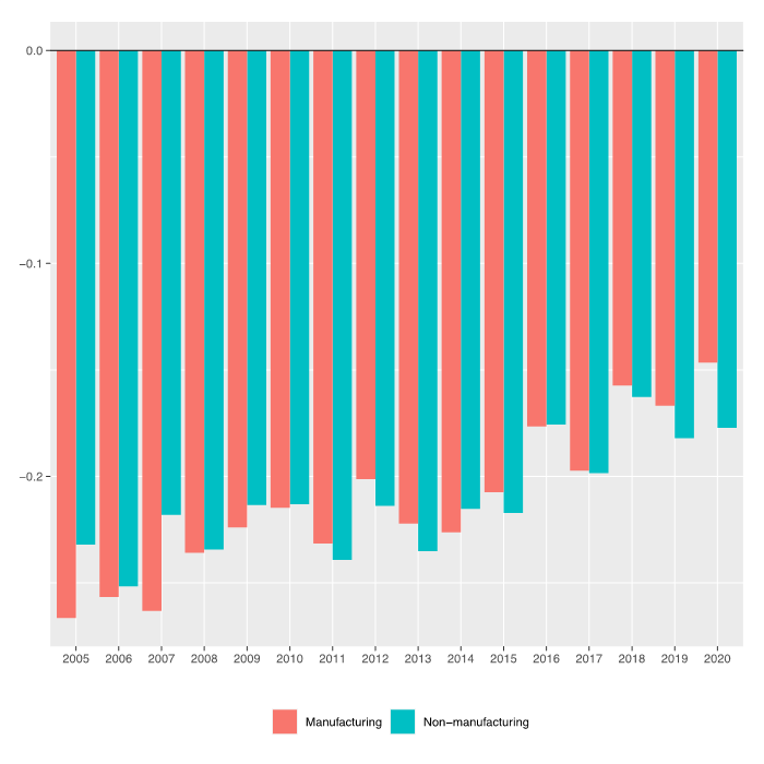
Figure 27. Working poverty differentials for informal workers (i-WPRE) (weighted average informal–formal differentials for manufacturing and non-manufacturing industries, four-digit NAICS level)
Note: Weights are equal to the inverse of the variance of the corresponding estimated coefficients.
Figure 28. Low pay rate differentials for informal workers (i-ELPR) (weighted average informal–formal differentials for manufacturing and non-manufacturing industries, four-digit NAICS level)
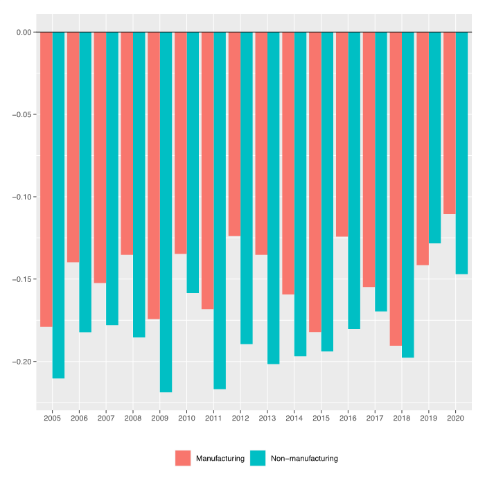
Note: Weights are equal to the inverse of the variance of the corresponding estimated coefficients.
Figure 29. Share of imported inputs in total inputs (
Note: Weights are equal to the inverse of the variance of the corresponding estimated coefficients.
Figure 30. Share of exports in total net sales (
Note: Weights are equal to the inverse of the variance of the corresponding estimated coefficients.
Table 1. Annual mean values of establishment-level variables
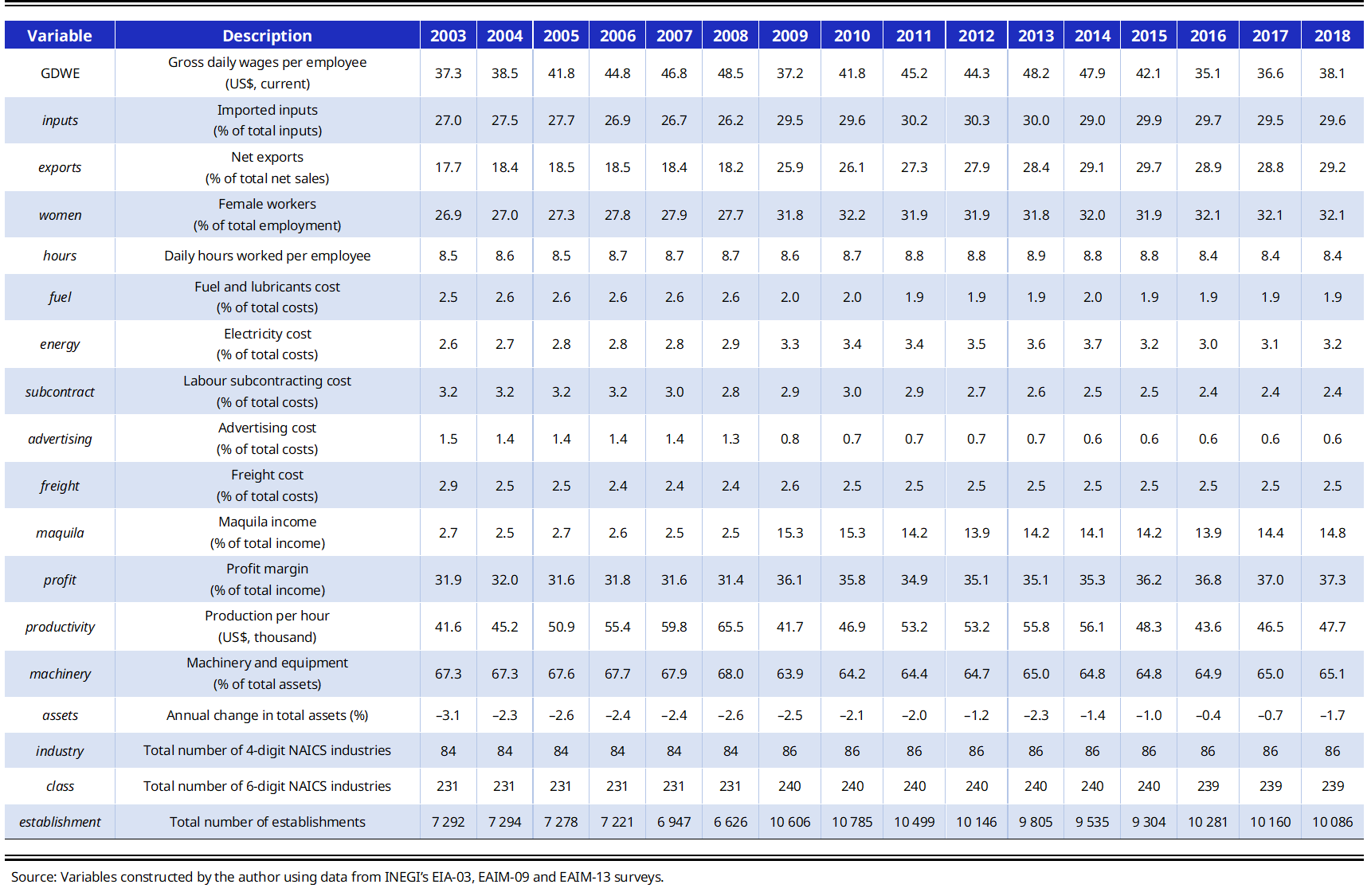
Table 2. Annual mean values of worker-level variables
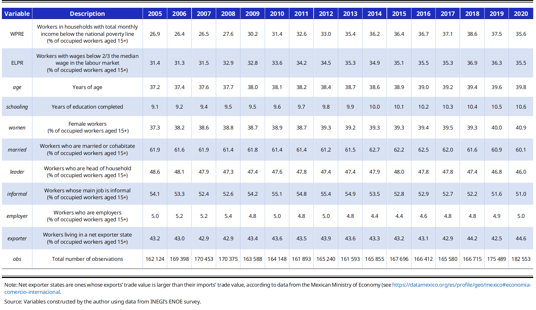
Table 3. Panel data models for ln(GDWE)
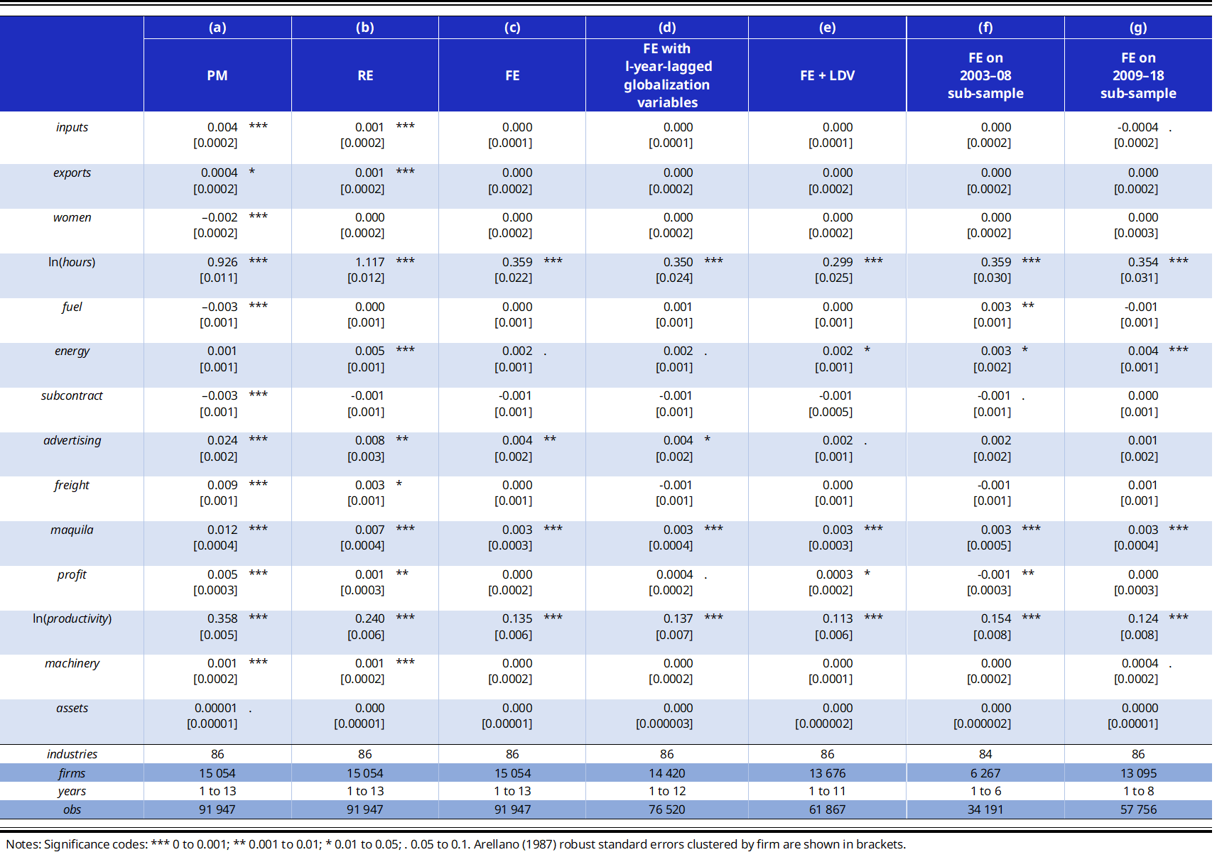
Table 4. Linear probability model for working poverty of employed persons (WPRE)
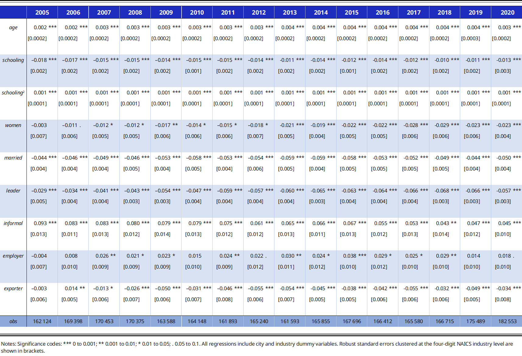
Table 5. Linear probability model for employees with low pay rate (ELPR)
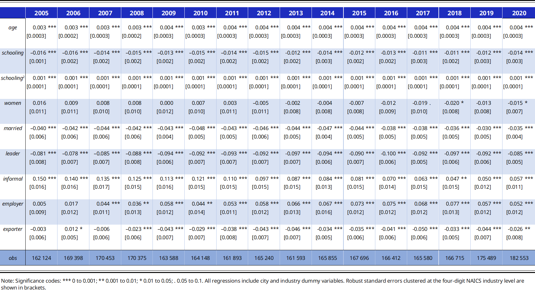
Table 6. Linear probability model for informal workers in working poverty (i-WPRE)
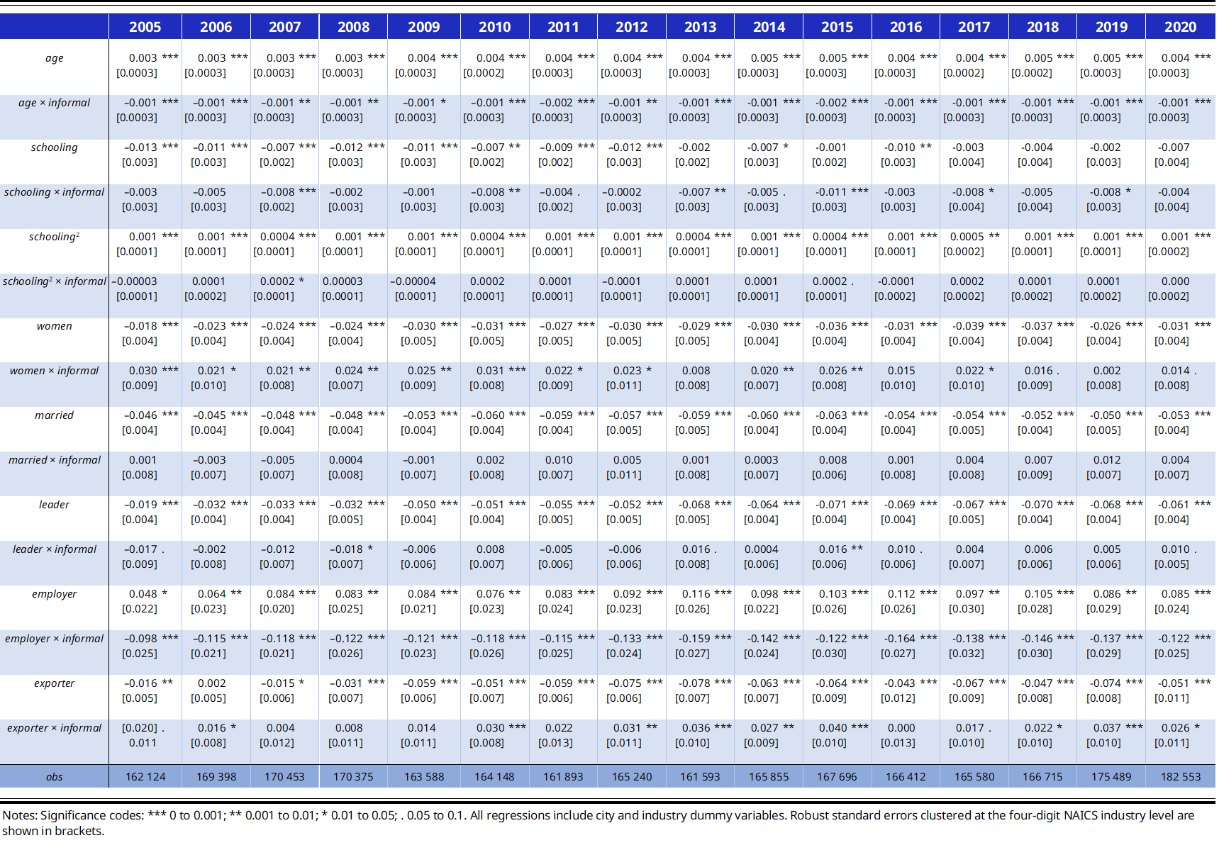
Table 7. Linear probability model for informal employees with low pay rates (i-ELPR)
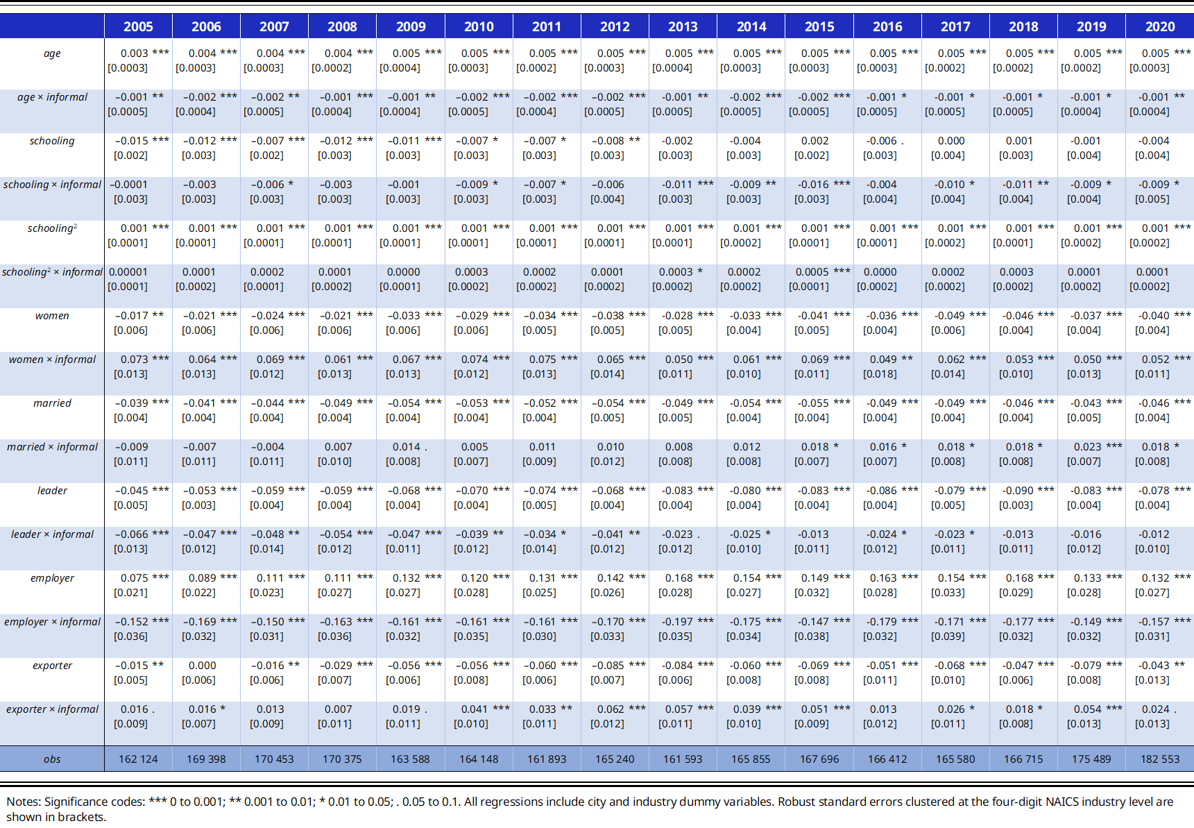
Table 8. Linear model for share of imported inputs in total inputs (
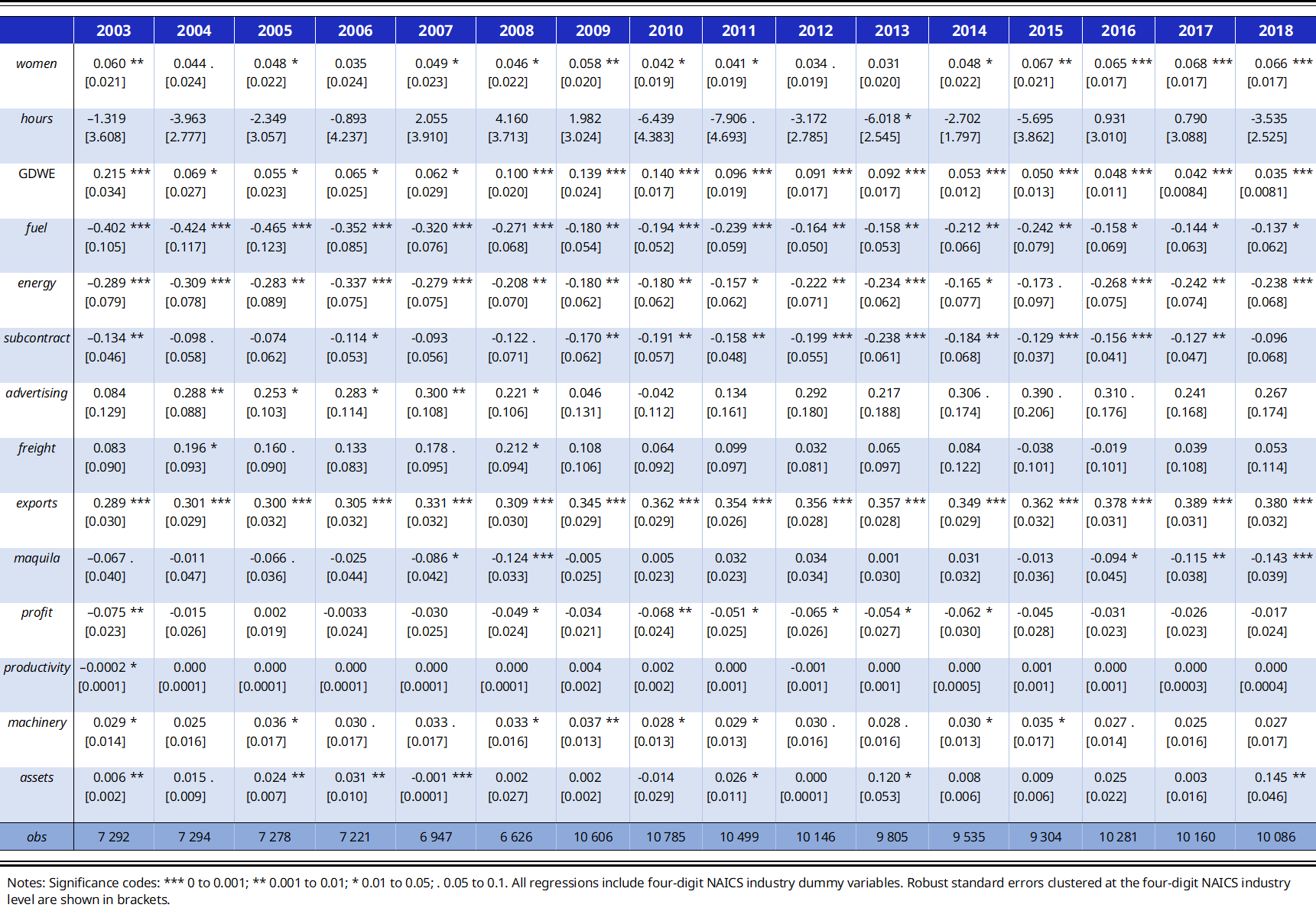
Table 9. Linear model for share of exports in total sales (
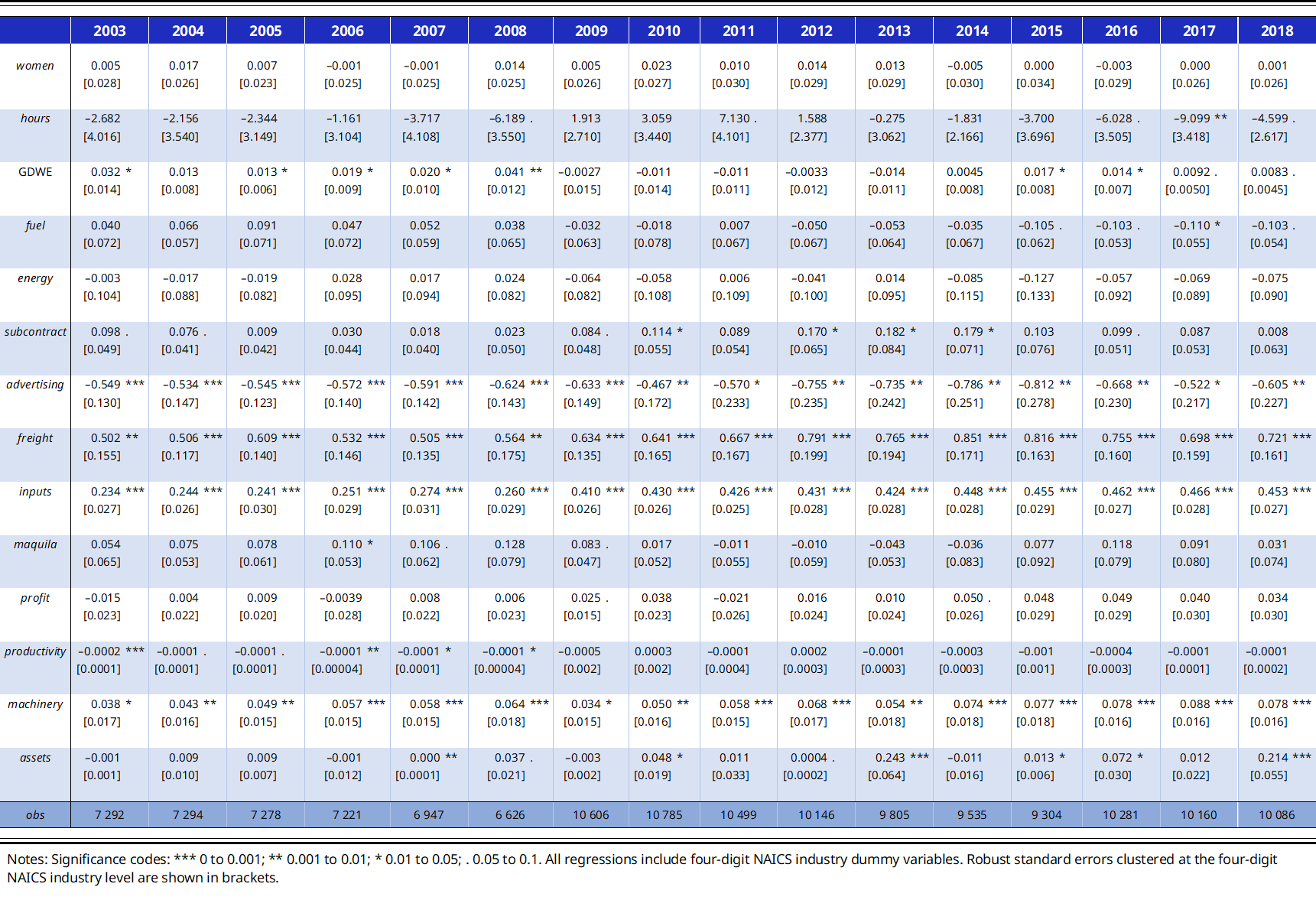
Table 10. Effect of non-preferential trade liberalization and exposure to globalization on working poverty and low pay rates
References
Abowd, J.A., F. Kramarz, and S. Woodcock. 2008. “Econometric Analyses of Linked Employer–Employee Data”. In
Aleman-Castilla, Benjamin. 2006. “The Effect of Trade Liberalization on Informality and Wages: Evidence from Mexico”, CEP Working Paper WP763 (October).
———. 2020. “Trade and Labour Market Outcomes: Theory and Evidence at the Firm and Worker Levels”, ILO Working Paper 12.
Aleman-Castilla, Benjamin, and Karla Cuilty-Esquivel. 2020. “Trabajo Decente En México, 2005–2020: Análisis Con Perspectiva de Género”. Unpublished. Mexico City: Centro de Investigación de la Mujer en la Alta Dirección, IPADE Business School.
Alfaro-Urena, A., I. Manelici, and J.P. Vásquez. 2019. “The Effects of Multinationals on Workers: Evidence from Costa Rica”. Unpublished. http://files/503/Alfaro-Urena et al. - 2019 - The Effects of Multinationals on Workers Evidence.pdf.
Angrist, J.D., and J.S. Pischke. 2009.
Arellano, M. 1987. “Computing Robust Standard Errors for Within-Groups Estimators”.
Autor, D., D. Dorn, and G. Hanson. 2013. “The China Syndrome: Local Labor Market Effects of Import Competition in the United States”.
Ben Salem, M., and C. Zaki. 2019. “Revisiting the Impact of Trade Openness on Informal and Irregular Employment in Egypt”.
Ben Yahmed, S. 2017. “Gender Wage Discrimination and Trade Openness. Prejudiced Employers in an Open Industry”. ZEW Discussion Paper 17-047.
Bhagwati, J., and T.N. Srinivasan. 2002. “Trade and Poverty in the Poor Countries”.
Bryson, A., J. Forth, and C. Barber. 2006. “Making Linked Employer–Employee Data Relevant to Policy”, DTI Ocassional Paper 4.
CONEVAL (National Council for Evaluation of Social Development Policy). 2020a. “Índice de La Tendencia Laboral de La Pobreza (ITLP): Resultados Nacionales y Por Entidad Federativa, Noviembre 2020”. Mexico City.
———. 2020b. “Líneas de Pobreza Por Ingresos”. InfoPobreza.
Coşar, A. Kerem, Nezih Guner, and James Tybout. 2016. “Firm Dynamics, Job Turnover, and Wage Distributions in an Open Economy”.
Cruces, G., G. Porto, and M. Viollaz. 2018. “Trade Liberalization and Informality in Argentina: Exploring the Adjustment Mechanisms”, CEDLAS Working Paper 0229.
Dix-Carneiro, R., P.K. Goldberg, Costas Meghir, and G. Ulyssea. 2021. “Trade and Informality in the Presence of Labor Market Frictions and Regulations”, NBER Working Paper 28391.
Dix-Carneiro, Rafael, and Brian K. Kovak. 2017. “Trade Liberalization and Regional Dynamics”.
———. 2019. “Margins of Labor Market Adjustment to Trade”.
Edmonds, E.V., N. Pavcnik, and P. Topalova. 2010. “Trade Adjustment and Human Capital Investments: Evidence from Indian Tariff Reform”.
Feenstra, R.C., R. Inklaar and M.P. Timmer. 2015. "The Next Generation of the Penn World Table".
Goldberg, P.K., and N. Pavcnik. 2003. “The Response of the Informal Sector to Trade Liberalization”.
Gourieroux, Christian, Alberto Holly, and Alain Monfort. 1982. “Likelihood Ratio Test, Wald Test, and Kuhn–Tucker Test in Linear Models with Inequality Constraints on the Regression Parameters”.
Government of Canada. 2020. “Comprehensive and Progressive Agreement for Trans-Pacific Partnership (CPTPP)”. https://www.international.gc.ca/trade-commerce/trade-agreements-accords-commerciaux/agr-acc/cptpp-ptpgp/index.aspx?lang=eng#:~:text=The Comprehensive and Progressive Agreement,%2C Peru%2C Singapore and Vietnam.
Hakobyan, S., and J. McLaren. 2017. “NAFTA and the Gender Wage Gap”, Upjohn Institute Working Paper 17–270.
Hausman, J.A. 1978. “Specification Tests in Econometrics”.
Helpman, E., O. Itskhoki, M.A. Muendler, and S.J. Redding. 2017. “Trade and Inequality: From Theory to Estimation”.
ILO. 1999.
———. 2008.
———. 2013. “Decent Work Indicators: Guidelines for Producers and Users of Statistical and Legal Framework Indicators”.
———. 2020.
———. 2021.
INEGI. 2007.
———. 2012.
———. 2015.
———. 2019.
———. 2020.
Jensen, P H. 2010. “Exploring the Uses of Matched Employer–Employee Datasets”.
Juhn, C., U. Gergely, and C. Villegas-Sanchez. 2014. “Men, Women, and Machines: How Trade Impacts Gender Inequality”.
Kis-Katos, K., and R. Sparrow. 2011. “Child Labor and Trade Liberalization in Indonesia”.
Kovak, B. 2013. “Regional Effects of Trade Reform: What Is the Correct Measure of Liberalization?”
Krishna, Pravin, Jennifer Poole, and Mine Senses. 2014. “Wage Effects of Trade Reform with Endogenous Worker Mobility”.
Lee, H., and J. Lee. 2015. “The Impact of Offshoring on Temporary Workers: Evidence on Wages from South Korea”.
Liang, Kung-Yee, and Scott L. Zeger. 1986. “Longitudinal Data Analysis Using Generalized Linear Models”.
Matthee, M., N. Rankin, and C. Bezuidenhout. 2017. “Labour Demand and the Distribution of Wages in South African Manufacturing Exporters”, WIDER Working Paper 2017/11.
Melitz, M.J. 2003. “The Impact of Trade on Intra-industry Reallocations and Aggregate Industry Productivity”.
Mitra, Devashish. 2016. “Trade Liberalization and Poverty Reduction”.
Mittag, N. 2019. “A Simple Method to Estimate Large Fixed Effects Models Applied to Wage Determinants”.
Ohlin, B. 1933.
Olarreaga, Marcelo, Gady Saiovici, and Cristian Ugarte. 2020. “Child Labour and Global Value Chains”, CEPR Discussion Paper DP15426.
Sampson, Thomas. 2014. “Selection into Trade and Wage Inequality”.
Sánchez Gómez, Joaquín, Juan Carlos Moreno-Brid, Lizzeth Gómez Rodríguez, and Rosa Gómez Tovar. 2021. “Trade Liberalization, Labor Market Outcomes and Decent Work in Mexico: The Case of the Automotive and the Textile Industries”, ILO Working Paper.
Schank, Thorsten, Claus Schnabel, and Joachim Wagner. 2007. “Do Exporters Really Pay Higher Wages? First Evidence from German Linked Employer-Employee Data”.
Schröder, S. 2018. “Wage Inequality and the Role of Multinational Firms: Evidence from German Linked Employer–Employee Data”. University of Edinburgh.
Secretaría de Economía. 2016. “Información Sobre Tratados Internacionales Que México Ha Suscrito En El Mundo”, Sistema de Información de Tratados Comerciales Internacionales (SICAIT).
Ulyssea, Gabriel, and Vladimir Ponczek. 2018. “Enforcement of Labor Regulation and the Labor Market Effects of Trade: Evidence from Brazil”. IZA Discussion Paper 11783.
UN. 2008.
Verhoogen, E.A. 2008. “Trade, Quality Upgrading, and Wage Inequality in the Mexican Manufacturing Sector”.
Woodcock, S. 2015. “Match Effects”.
World Bank Group, and WTO (World Trade Organization). 2015.
———. 2018.
Yeaple, S. 2005. “A Simple Model of Firm Heterogeneity, International Trade, and Wages”.
Acknowledgements
I am very grateful to Marva Corley-Coulibaly and Pelin Sekerler Richiardi, of the ILO Research Department, for the opportunity to collaborate in the project “Trade, enterprises and labour markets: Diagnostic and firm level assessment”, conducted jointly by the European Commission and the ILO. I am also grateful to Ira Postolachi, Sajid Ghani, Mónica Hernández, Marc Bacchetta, Marva Corley-Coulibaly, Pelin Sekerler Richiardi and participants at the ILO Research BBL (Brown Bag Lunch) webinar for their very useful comments; and to Angela Doku, Béatrice Guillemain, Sarah Álvarez, Anthony Nanson and Natalia Volkow and INEGI’s Microdata Lab team for their administrative and technical support. Any errors that remain are my own.

