Global Wage Report 2022–23
The impact of inflation and COVID-19 on wages and purchasing power

4. Wage inequality in the context of the COVID-19 crisis and rising price inflation

Wage inequality, together with other labour income inequalities, is a major contributor to total income inequality between households and thus an important factor behind income inequality at the country level (ILO 2021b). It is therefore relevant for policymakers to consider, on the basis of empirical data, how wage inequality may have changed in recent times and the role played by the ongoing crises in shaping these changes.

This chapter starts by presenting wage inequality estimates based on data from before the COVID-19 pandemic (2019) and comparing these with estimates based on more recent data (2021 or 2022). It then seeks to decompose the changes in wage inequality so as to disentangle the contribution due to a change in the composition of wage employees from the contribution due to structural changes in the wage distribution. The last section presents estimates that show the change in the gender pay gap since the outbreak of the pandemic, emphasizing that the pay gap between women and men continues to be an important factor behind wage inequality.

The pay gap between women and men continues to be an important factor behind wage inequality

.4.1. The COVID-19 crisis and wage inequality

Figure 4.1 compares estimates of wage inequality between 2019 and 2021 (or 2022) using six differ- ent inequality indicators for 22 countries for which data are available.1 The use of several indicators (see box 4.1 for the definitions of these) makes it possible to construct a more detailed picture of changing wage inequality. While the Palma ratio and the Gini coefficient each compare the accumu- lation of earnings across the wage distribution, in- dicators based on the ratio of wages at two decile thresholds compare different locations of the wage distribution. In this report, the Palma ratio and the Gini coefficient are estimated using monthly earn- ings, whereas the decile ratios D9/D1, D9/D5, D8/D2 and D5/D1 are estimated using the distribution of hourly wages. For example, D9/D1 measures the ra- tio of the threshold of the top decile (D9) to that of the bottom decile (D1) in the distribution of hourly wages. Because monthly earnings take into account both hourly wages and hours worked, comparing changes in wage inequality as captured by indica- tors that use monthly earnings with changes cap- tured by indicators that use hourly wages can shed light on how changes in working time shape wage inequality. Table 4.1 complements figure 4.1, which shows the change in wage inequality between periods, by providing a summary of the extent to which each of the six measures of wage inequality has changed in each of the 22 countries.2

As can be seen from figure 4.1 and table 4.1, there are similarities between estimates using the Palma ratio and the Gini coefficient. In 10 of the 22 countries, monthly wage inequality increased (visibly more in Colombia, Panama, Paraguay and Thailand), while in the remaining 12 countries wage inequality dropped (visibly more in the Plurinational State of Bolivia, the Dominican Republic, Peru and the United States). Colombia and Panama stand out as the two countries with the greatest increase in wage inequality between 2019 and 2021 (2022 in the case of Colombia). Peru is the country where wage inequality decreased the most between 2019 and 2022: the Palma ratio shows that in 2019 the top 10 per cent accumulated 100 per cent more in monthly earnings than the bottom 40 per cent, while in 2022 the gap dropped to 72 per cent. For most other countries the change in wage inequality in the three years is small. Table 4.1 shows that in 16 of the 22 countries the magnitude of the change in the Gini coefficient is less than 6 per cent, while in some of these countries (for example, Ecuador, Indonesia, Mexico and the Philippines) it is less than 1 per cent. Countries that exhibit a large increase in wage inequality could take a long time to achieve more equitable wage structures, hence the need for suitable policies (see Chapter 5). In countries where the Gini coefficient or the Palma ratio indicates a substantial drop in wage inequality, the estimates could well be masking composition effects – this will be explored further in section 4.2.

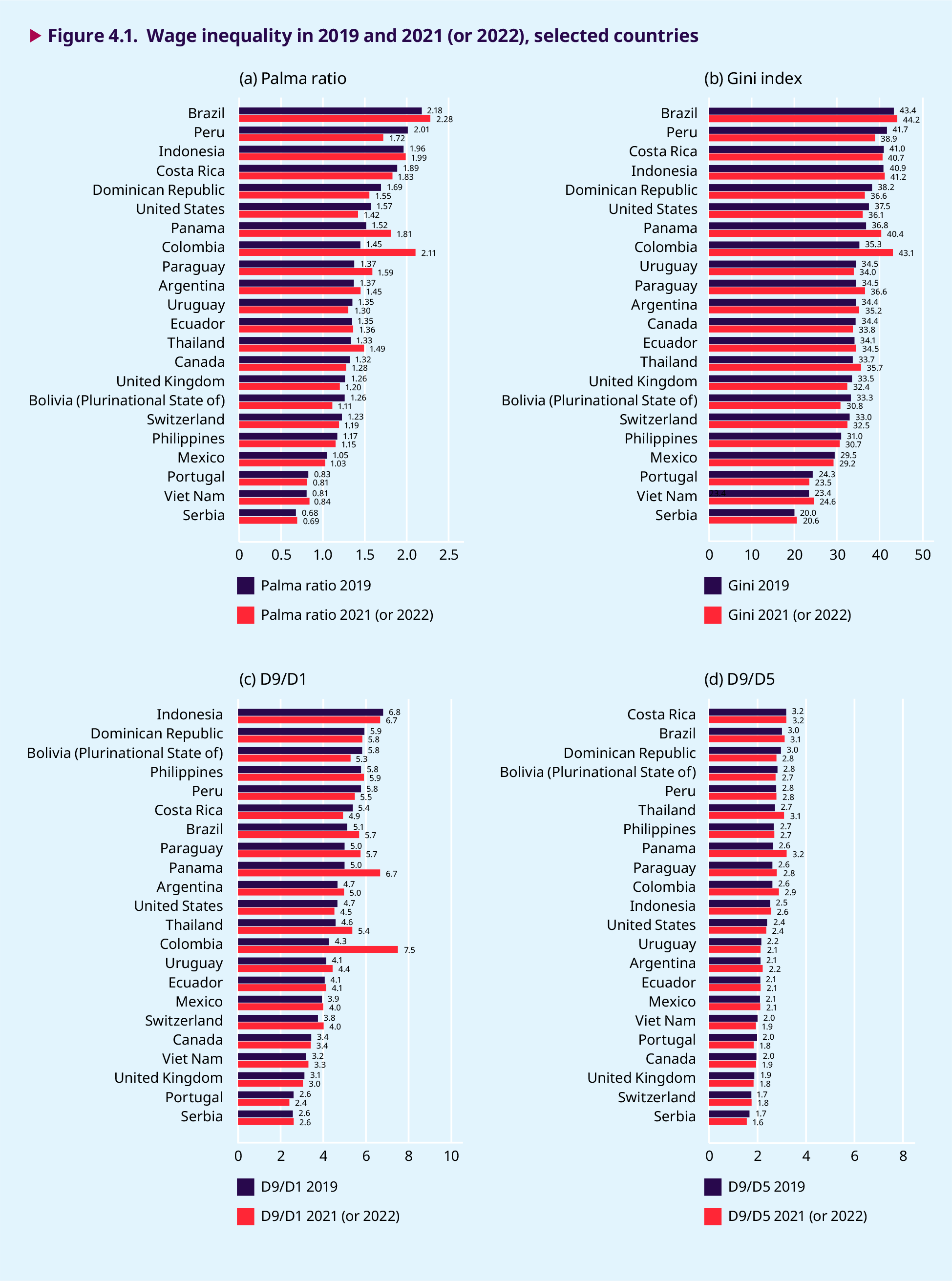
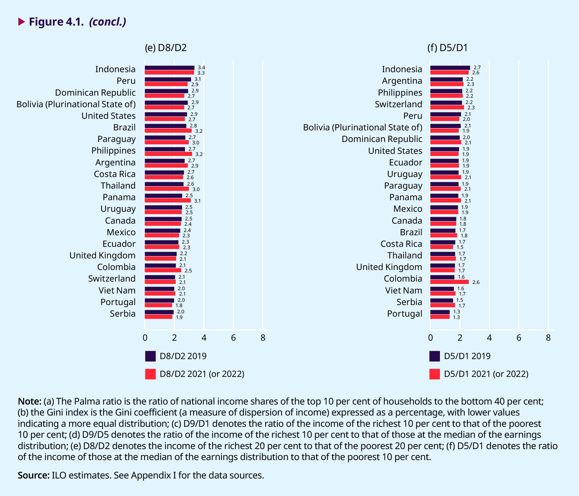
Estimates of wage inequality using decile ratios, (charts (c) to (f) in figure 4.1) are useful in detect- ing whether specific locations of the wage dis- tribution are shaping the overall change in wage inequality. For example, in Colombia, the large in- crease in wage inequality seems to be driven by a distancing of the bottom decile from other de- ciles in the distribution of hourly wages. This can be seen because the increases in the D9/D1 and D5/D1 ratios between 2019 and 2022 are striking- ly large, whereas the D8/D2 and D9/D5 ratios have increased by much less. In contrast, in Panama, the D9/D1, D8/D2 and D9/D5 ratios have increased similarly, whereas the change in the D5/D1 ratio is much smaller. Therefore, in Panama, the country that shows the greatest increase in wage inequality together with Colombia, the increase between 2019 and 2022 seems to be driven by a widening of the wage distribution at the top: the threshold value for the hourly wages of the top decile has increased.

Changes in wage inequality can result from a mixture of changes in working time, changes in the earnings from time worked and changes affecting specific regions of the wage distribution.

Table 4.1. Percentage change in wage inequality, selected countries, 2019–21 or 2019–22

Note: The countries have been organized by ascending order of change in wage inequality, as measured by the Palma ratio, between 2019 and 2021 (or 2022). A negative value indicates a decline in wage inequality between periods, while a positive value indicates an increase. For example, in Colombia, the country with the largest increase in the Palma ratio and therefore placed at the bottom of the table, the Palma ratio in 2019 was estimated at 1.45, meaning that the top 10 per cent of wage employees accumulated 45 per cent more total earnings than the bottom 40 per cent in the first quarter of 2019. In 2022 (first quarter) the Palma ratio had increased to 2.11, that is, the top 10 per cent accumulated 111 per cent more than the bottom 40 per cent. The increase between the estimate of 1.45 in 2019 and the estimate of 2.11 in 2022 is approximately 45.5 per cent.

Source: ILO estimates. See Appendix I for the data sources.

Understanding the complex structure of changes in wage inequality is a prerequisite for designing policies to reduce such inequality.

In 4 of the 22 countries, wage inequality as measured by monthly earnings (the Palma ratio or the Gini coefficient) has changed in the opposite direction to that of the change in wage inequality as estimated using ratios between pairs of deciles at their thresholds in the distribution of hourly wages. In Mexico, the Philippines and Switzerland the four decile ratios suggest that wage inequality has increased across the distribution, since for all three countries the changes in the ratios between 2019 and 2021 (or 2022) are positive. However, in all three countries the Palma ratio and the Gini coefficient are negative. This could indicate that despite increasing inequality in hourly wages, the number of hours worked has changed – increasing on average among lower earners and/or decreasing on average among higher earners – thereby leading to a drop in overall inequality in monthly earnings. In Indonesia the opposite is true: hourly wage inequality has declined across the wage distribution, but changes in the pattern of hours worked among top and bottom earners have led to increasing inequality in monthly earnings.

For all other countries in figure 4.1 and table 4.1 there is consistency between the six estimates of wage inequality: countries exhibiting an increase or a decrease in the Palma ratio and the Gini coefficient between 2019 and 2021 (or 2022) also exhibit an increase or a decrease, respectively, in the ratios of the various pairs of decile thresholds. However, analysis of these indicators shows that changes in wage inequality can result from a mixture of changes in working time, changes in the earnings from time worked and changes affecting specific regions of the wage distribution, particularly the extremes. Understanding the complex structure of changes in wage inequality is a prerequisite for designing policies to reduce such inequality.

.4.2. Uncovering the factors behind changes in wage inequality

During labour market shocks, wage inequality can change significantly because of composition effects associated with wage employment. For example, as a result of the COVID-19 crisis, many countries experienced massive job losses among the low- paid, particularly in the second and third quarters of 2020. These losses, clearly a negative labour market outcome by any measure, would never- theless have compressed the wage distribution at the bottom, thus reducing wage inequality at that time. In addition to composition effects, structur- al shifts can also change wage inequality. For ex- ample, the implementation of a minimum wage can compress the wage distribution from below, thereby reducing wage inequality without chang- ing the composition of wage employees (unless the During the COVID-19 crisis, the composition of wage employment was observed to have changed in relation to three of these characteristics: sex, economic sector and occupational category (ILO 2020c). Thus, the shares of female (and male) wage employees changed during and in the aftermath of the COVID-19-related restrictions, probably because women tend to be over-represented in low-paid jobs involving face-to-face work. (As already discussed in section 3.8, women’s share of employment losses was greater than that of men in several countries.) Similarly, some economic sectors (particularly the service sector, manufacturing and construction) and occupational categories (notably lower-skilled and unskilled occupations) were found minimum wage has a negative employment effect). Given that composition effects are often transito- ry, while structural changes tend to be more per- sistent, disentangling the factors that lie behind an overall change in wage inequality can be a useful tool for policymakers.

The composition of wage employees, and how it changes over time, is a complex outcome that reflects their multiple characteristics and circumstances. During the COVID-19 crisis, the composition of wage employment was observed to have changed in relation to three of these characteristics: sex, economic sector and occupational category (ILO 2020c). Thus, the shares of female (and male) wage employees changed during and in the aftermath of the COVID-19-related restrictions, probably because women tend to be over-represented in low-paid jobs involving face-to-face work. (As already discussed in section 3.8, women’s share of employment losses was greater than that of men in several countries.) Similarly, some economic sectors (particularly the service sector, manufacturing and construction) and occupational categories (notably lower-skilled and unskilled occupations) were found to be at greater risk of employment loss than others during the crisis (ILO 2020c). Building on the above observations, this section decomposes the change in wage inequality by examining the extent to which changes related to each of these three characteristics of wage employees contributed to the observed change in wage inequality between 2019 and 2021 (or 2022). The method is based on DiNardo, Fortin and Lemieux (1996) and on Daly and Valletta (2006); Appendix V provides further details.

During labour market shocks, wage inequality can change significantly because of composition effects associated with wage employment.

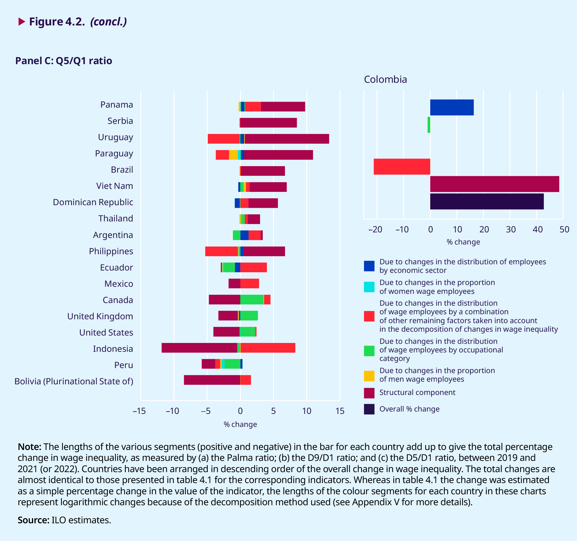
Figure 4.2 presents a decomposition of changing wage inequality that considers changes in the Palma ratio, the D9/D1 ratio and the D5/D1 ratio.3 In each of the three charts, and for each country, the differently coloured segments of each bar, which may indicate negative or positive values, add up to the total percentage change in wage inequality between 2019 and 2021 (or 2022). These totals correspond to the values given in table 4.1. Whereas the contributions due to the three worker characteristics mentioned above are shown separately, the contribution to changing wage inequality resulting from compositional changes in “other factors” is shown in a single colour segment.4 When a segment appears to the right of zero, it means that changes in the composition of the corresponding factor between 2019 and 2021 (or 2022) have contributed to an increase in wage inequality over that period; when a segment appears to the left of zero, the change in the corresponding factor has contributed to a reduction in wage inequality over that period. Structural change can also contribute to changes in wage inequality: as with each of the compositional factors, it can either increase or decrease inequality and so the relevant colour segment in each bar will appear either to the right or the left of zero, as the case may be. In all three charts in figure 4.2, the results of the decomposition for Colombia are displayed separately. This is to prevent the scale required to show the very large changes estimated for Colombia from blurring the presentation of the other countries.

In addition to composition effects, structural shifts – such as the implementation of a minimum wage – can also change wage inequality.

The three charts in figure 4.2 show similarities in terms of how the various factors may have contributed to the compositional component of the total change in wage inequality. The variables that were considered separately (sex, economic sector and occupational category) do not appear to have had a decisive influence on the total change in wage inequality, especially compared with the role of the mixed “other factors”. In particular, changes in the relative share of women and men in the population of wage employees do not seem to play an important role. A detailed inspection of the microdata reveals that, among the 19 countries covered by figure 4.2, the shares of female and male wage employees in 2021 (or 2022) are almost identical to those observed in 2019. Some countries exhibit a slight increase in the share of men, but it is less than 2 per cent in all cases. It seems, therefore, that women gradually returned to their pre- pandemic employment levels. This means that when wage inequality is measured in 2021 (2022), relative to 2019, the gender composition of the workforce does not emerge as a relevant factor when it comes to explaining observed changes in wage inequality.

Disentangling the factors that lie behind an overall change in wage inequality can be a useful tool for policymakers.

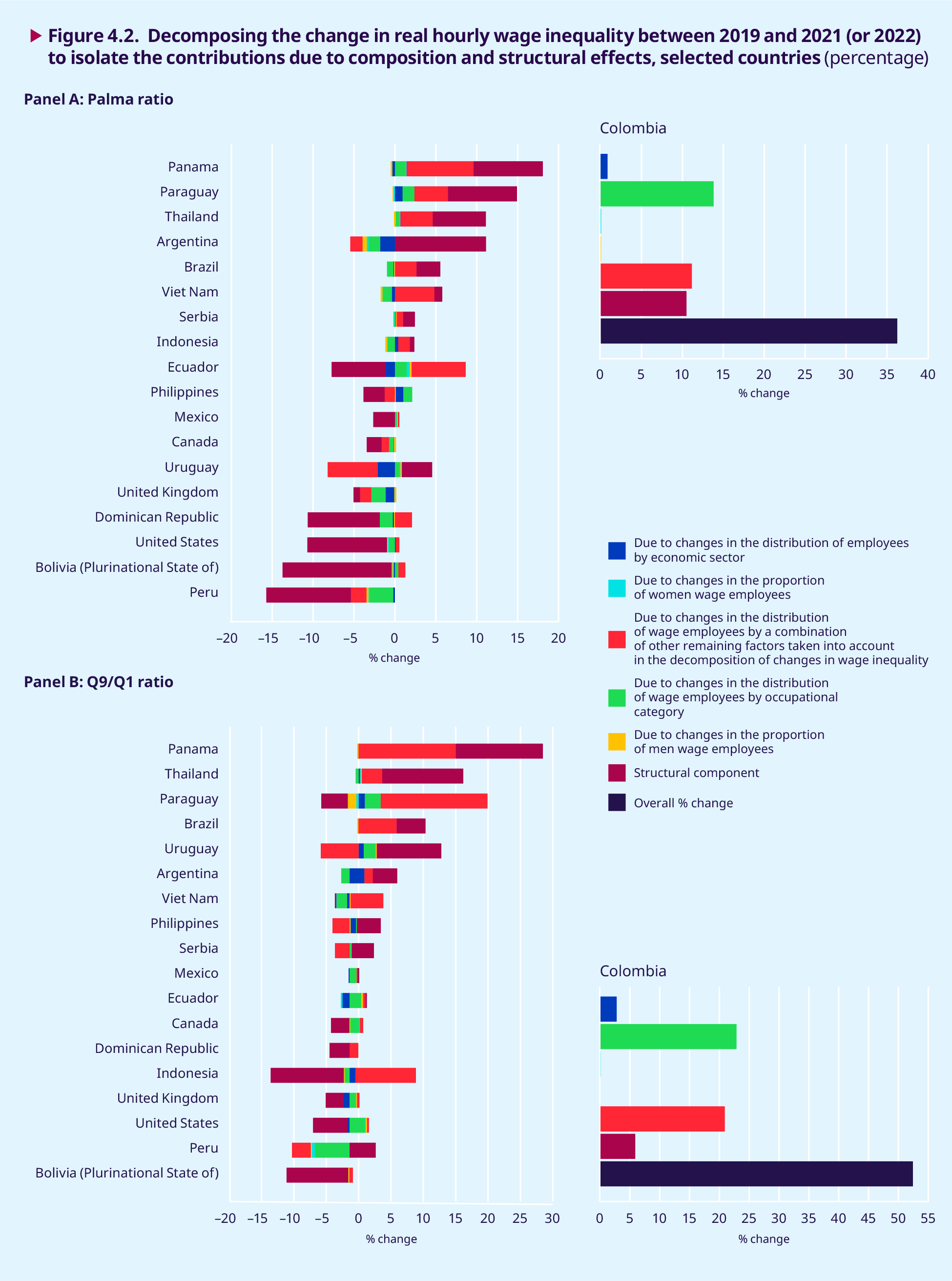
In comparison to gender composition, changes in the relative shares of wage employees by economic sector and occupational category seem to be slight- ly more relevant as drivers of changes in wage in- equality. For example, in Argentina, the change in the relative share of wage employees by economic sector increased wage inequality by 2.4 per cent when measured using the D9/D1 ratio, with the overall increase in wage inequality during the rele- vant period estimated at 6.6 per cent. This means that had the relative share of wage employees by economic sector remained as in 2019 at the ex- treme deciles of the wage distribution, the D9/D1 ratio would have increased by 4.1 per cent, rather than by 6.6 per cent (all other things being equal). When the Palma ratio is used, the factor “economic sector” contributes negatively to changing wage in- equality in Argentina. Thus, the relative shares, by economic sector, of the top 10 per cent and the bot- tom 40 per cent of earners changed between 2019 and 2021 in such a way that inequality as meas- ured by the Palma ratio decreased by 1.8 per cent. Apart from Argentina – and possibly Uruguay as well – the factor “economic sector” does not seem to play a significant role in driving changes in in- equality among the countries studied. Compared with gender composition or economic sector, a change in the relative shares of wage employees by occupational category appears to be a more relevant contributor to changes in wage inequality. Looking at the Palma ratio, changes in the relative shares of the various occupational categories con- tributed to a noticeable increase in wage inequality in Colombia (14 per cent), Ecuador (1.5 per cent), Panama (1.4 per cent) and Paraguay (1.4 per cent), and to a noticeable drop in wage inequality in Argentina (–1.4 per cent), the Dominican Republic (–1.6 per cent), Indonesia (–1.1 per cent), Peru (–2.9 per cent), the United Kingdom (–1.8 per cent) and Viet Nam (–1.2 per cent).

In general, the charts in figure 4.2 show that despite the compositional changes in employment during the COVID-19 crisis in terms of occupations, economic sectors and the relative shares of female and male employees, at present, as the effect of the crisis on labour markets begins to fade, the composition effect behind changes in wage inequality is also diminishing. This finding is consistent with the transitory nature of composition effects during labour market shocks. In a few countries, the “other factors” group, which includes education, age and formality status, does seem to be a stronger determinant of changing wage inequality – and in most cases, changes in the composition of this mixed set of factors appear to have contributed to an increase in wage inequality. However, what is far more striking in figure 4.2 is that changes in wage inequality between 2019 and 2021 (or 2022) appear to be strongly driven by changes in the wage structure. Once compositional effects vanish altogether, structural changes are likely to continue shaping the wage distribution in the future. In some of the countries studied (for example, Argentina, Colombia, Panama, Paraguay and Thailand), this implies large increases in wage inequality.

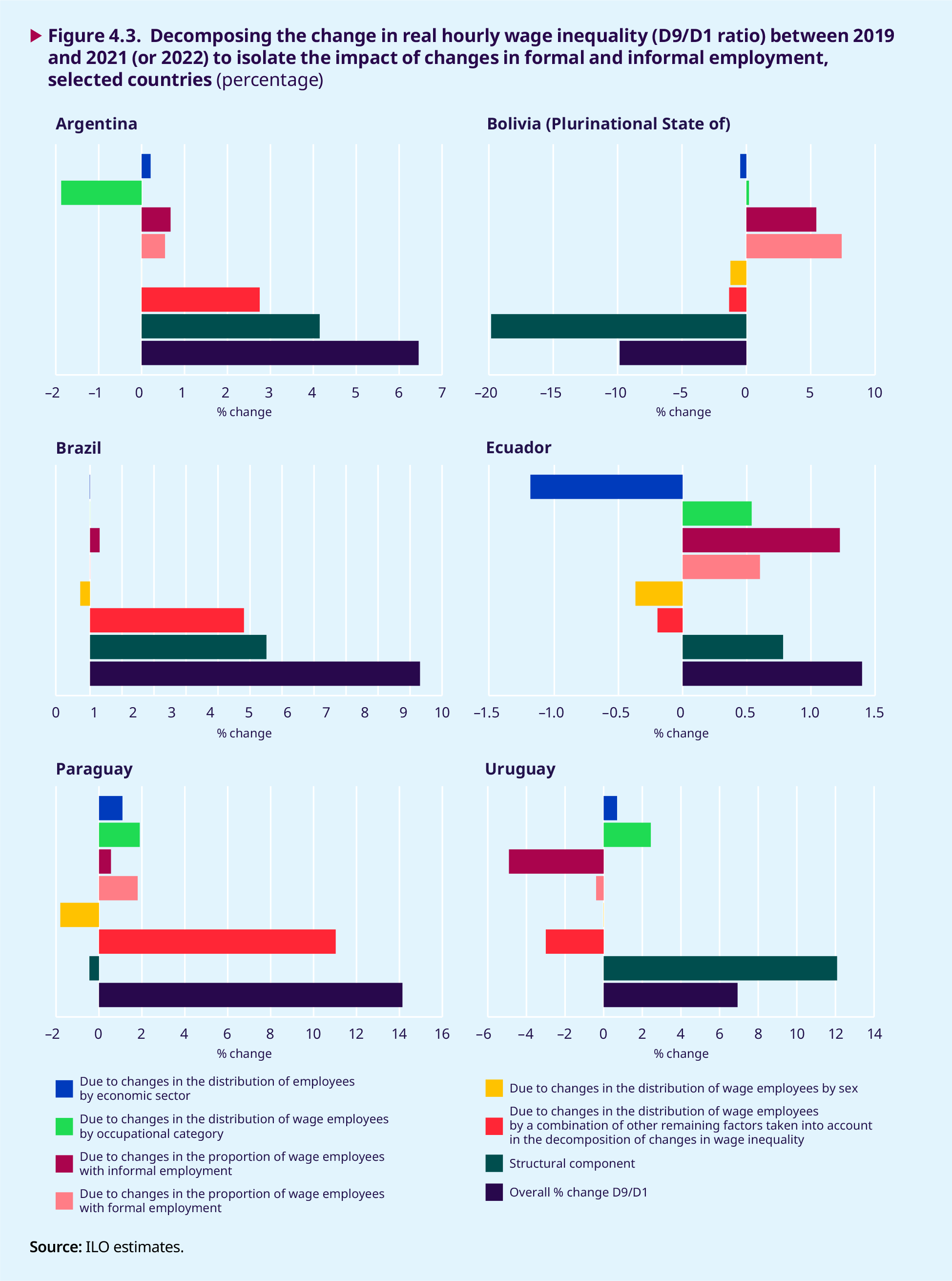
In most cases a change in the relative shares of formal and informal employment between 2019 and 2021 (or 2022) was associated with an increase in wage inequality.

Earlier in the report (see section 2.4) it was pointed out that as employment gradually recovers to pre- pandemic levels, in some countries – particularly those with large numbers of informal workers – informal employment is increasing at a faster rate than formal employment. Figure 4.3 is based on a similar decomposition exercise to that in figure 4.2, but it seeks instead to identify how changes in the relative shares of formal and informal employment influenced changes in wage inequality between 2019 and 2021 (or 2022). As can be seen, in most cases a change in the relative shares of formal and informal employment was associated with an increase in wage inequality. In Ecuador and Paraguay, where informality among wage employees rose by 7 per cent and 4 per cent, respectively, the increase in informal wage employment and concomitant decrease in formal employment contributed to an increase in wage inequality. In Uruguay, where the microdata show a 4 per cent decrease in informal wage employment (and a corresponding increase in formal employment), there was compression at the bottom of the wage distribution, reflecting a reduction in wage inequality. The findings from figure 4.3 serve to highlight the need for formalization of the informal economy.

.4.3. The COVID-19 crisis and the gender pay gap

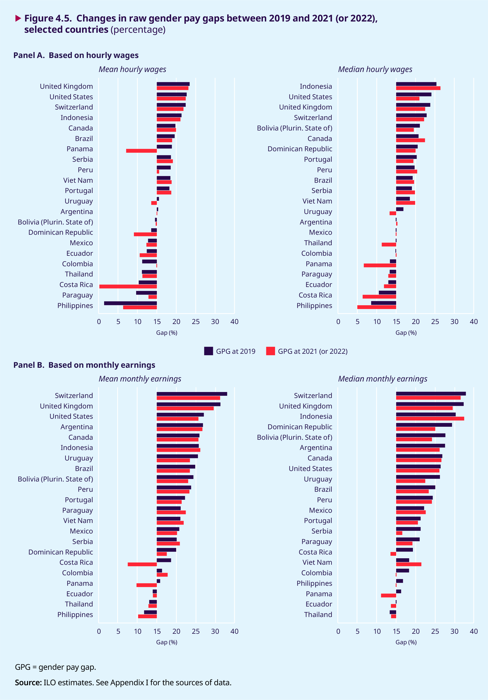
Did the COVID-19 health crisis contribute to a widening of the gender pay gap? Figure 4.4 presents estimates of the mean and median factor-weighted gender pay gaps between women and men for both hourly wages and monthly earnings. Factor- weighted gender pay gaps were first used in the Global Wage Report 2018/19 (ILO 2018). This method is an alternative to the traditional use of mean and median “raw” gender pay gaps, and eliminates potential bias due to the unequal clustering of women and men at different locations of the wage distribution (see box 4.2 for more details). Although this section relies on factor-weighted gender pay gaps to compare pay differentials between women and men, figure 4.5 complements the analysis by presenting the traditional raw mean and median gender pay gaps based on both hourly wages and monthly earnings.

Panels A and B in figure 4.4 present estimates of the factor-weighted gender pay gap for up to 22 countries for which comparable data for the period from 2019 to 2021 (or 2022) are available. When the factor-weighted method is used, as opposed to the traditional method of raw pay gaps underlying figure 4.5, all estimates of the hourly or monthly (mean or median) gender pay gaps are positive. This illustrates how, in many instances, use of the raw mean or median can give a misleading summary of the wage distribution for the purpose of comparing the earnings of women and men. Instead, the use of weighted averages of gender pay gaps between subgroups of women and men with similar labour market characteristics allows one to avoid underestimating or overestimating the pay gap in the population as a whole (see box 4.2). Thus, although figure 4.5 is included in this section for the sake of completeness, the analysis is centred on figure 4.4, which shows estimates of the factor-weighted gender pay gap.

The estimates presented in the Global Wage Report 2018/19 indicated a global average gender pay gap of about 20 per cent, based on data from 80 countries (ILO 2018). This edition examines the evolution of gender pay gaps in a more limited sample of countries, finding very little change between 2019 and 2021–22. The charts in figure 4.4 show that the gender pay gap is positive in all the countries studied and has remained so over time.5 Across these 22 countries, the factor-weighted mean gender pay gap using hourly wages in 2019 ranged from about 2 per cent (Paraguay) to about 22 per cent (Plurinational State of Bolivia), while in 2021 it ranged from 2 per cent (Costa Rica) to about 24 per cent (Indonesia). Thus, whereas in 2019 the simple average of the mean gender pay gap using hourly wages across the 22 countries was 12.8 per cent, in 2021–22 it was 12.3 per cent. Similar estimates are found for the factor-weighted median gender pay gap, with the simple average in 2019 and 2021–22 standing at 11.9 per cent and 11.7 per cent, respectively. The estimates based on monthly earnings in figure 4.4 are a few percentage points higher than those based on hourly wages: whereas in 2019 the simple average using factor- weighted mean monthly earnings was 17 per cent, the average using median values was 16 per cent. Overall, figure 4.4 suggests that the gender pay gap continues to persist in labour markets around the world, with women paid, on average, less than men.

A more detailed look at figure 4.4, panel A – complemented by table 4.2 – reveals that between 2019 and 2021 (or 2022) the gender pay gap based on factor-weighted mean hourly wages increased in 9 of the 22 countries, with the increases ranging from about 0.6 percentage points (for example, in Serbia) to as much as 6.3 percentage points (Paraguay). Among the 13 countries where the factor-weighted mean hourly gender pay gap declined, the decreases ranged from 0.3 percentage points in Colombia to 7.5 percentage points in Panama. Except for a few countries, there is consistency in the direction of the change (that is, the sign) of mean and median estimates between 2019 and 2021 (or 2022), whether hourly wages or monthly earnings are used. One exception, for example, is Peru: the factor-weighted mean gender pay gap using hourly wages declined by 5.12 percentage points between 2019 and 2022, but the median gap increased by 0.88 percentage points. Overall, the four charts in figure 4.4 show that gender pay gaps were not greatly altered by the COVID-19 crisis. While estimates using mean hourly wages indicate an average drop of 0.61 percentage points in the gender pay gap among the 22 countries between 2019 and 2021 (or 2022), those based on mean monthly earnings suggest an increase of less than 0.1 percentage points. The average change in the gender pay gap is similar if estimates based on median hourly wages and median monthly earnings are used: –0.19 percentage points and 0.21 percentage points, respectively.

The gender pay gap continues to persist in labour markets around the world, with women paid, on average, less than men.

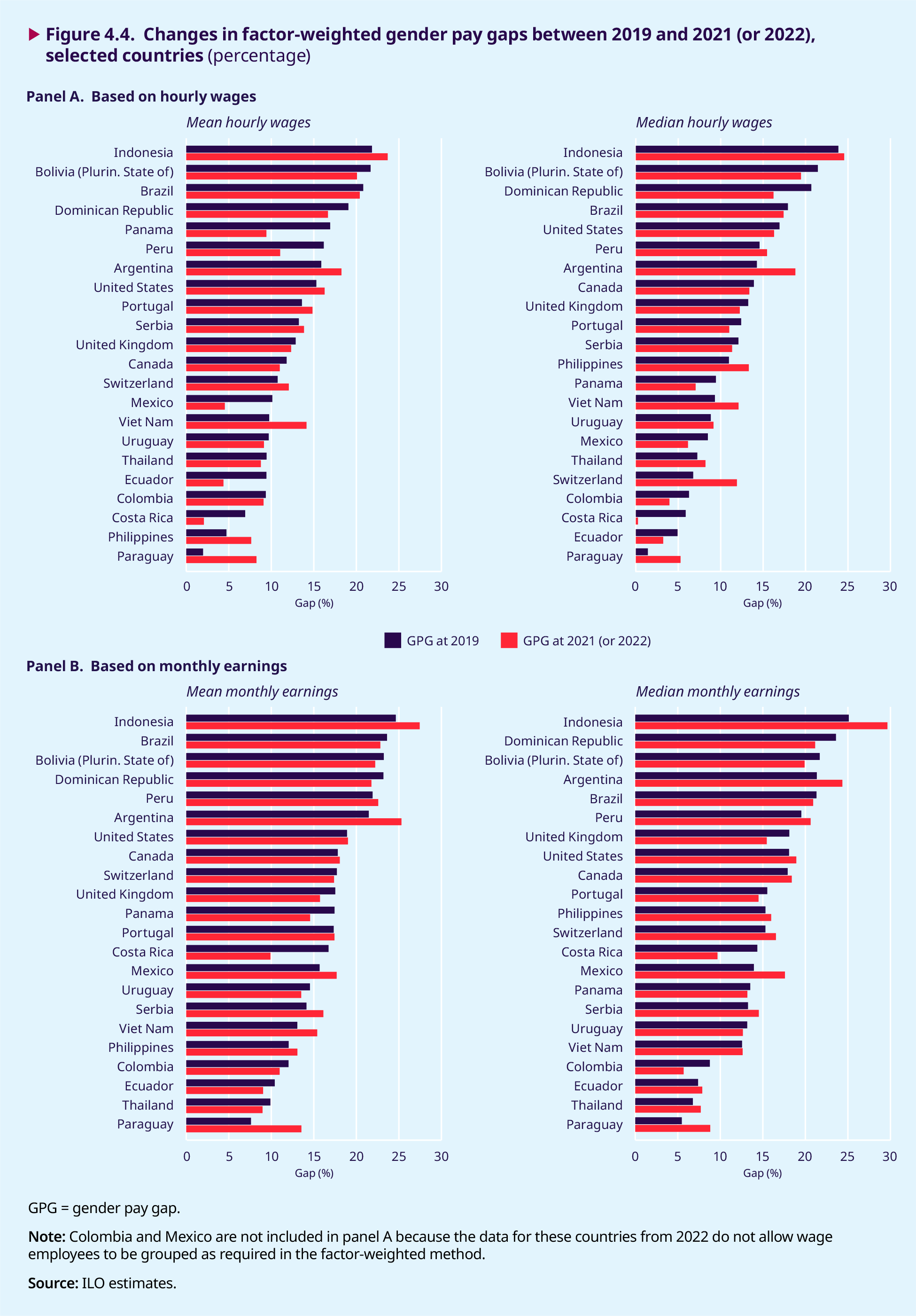
Table 4.2. Change in various measures of the factor-weighted gender pay gap between 2019 and 2021 (or 2022), selected countries (percentage points)

Note: The factor-weighted gender pay gap is calculated by clustering women and men into groups based on educational attainment, age, full-time versus part-time employment, and public versus private sector employment. For Paraguay, the Philippines and Uruguay, data related to educational attainment are not comparable between different years, and occupational sectors have been used instead to cluster women and men into homogenous groups. Colombia and Mexico had, respectively, 4 and 6 clusters (out of 64 possible clusters) in which a single person dominated the resulting pay gap.To avoid large variations, these clusters were excluded from the factor-weighted computation for both years. See box 4.2 for more details of how factor-weighted gender pay gaps are estimated.

Source: ILO estimates. See Appendix I for the data sources.

factor-weighted mean hourly gender pay gap declined, the decreases ranged from 0.3 percentage points in Colombia to 7.5 percentage points in Panama. Except for a few countries, there is consistency in the direction of the change (that is, the sign) of mean and median estimates between 2019 and 2021 (or 2022), whether hourly wages or monthly earnings are used. One exception, for example, is Peru: the factor-weighted mean gender pay gap using hourly wages declined by 5.12 percentage points between 2019 and 2022, but the median gap increased by 0.88 percentage points. Overall, the four charts in figure 4.4 show that gender pay gaps were not greatly altered by the COVID-19 crisis. While estimates using mean hourly wages indicate an average drop of 0.61 percentage points in the gender pay gap among the 22 countries between 2019 and 2021 (or 2022), those based on mean monthly earnings suggest an increase of less than 0.1 percentage points. The average change in the gender pay gap is similar if estimates based on median hourly wages and median monthly earnings are used: –0.19 percentage points and 0.21 percentage points, respectively.

Box 4.2. The factor-weighted gender pay gap: An illustrative example

Source: ILO estimates using national survey data from Egypt, 2012 (see ILO 2018a, Appendix V).

Source: Based on box 3 in ILO (2018).