Appendices

.Appendix I. Sources of quarterly survey data, spending patterns of households, and processing of the data

Sources of quarterly survey data

Processing of the survey data

In the above table, “Q” stands for “quarter” and “M” for “month”. Thus, “Q1 2019” denotes the first quar- ter of 2019 and “M1 2019” denotes January 2019.

• For all estimates, the first quarter (or month or year) in the data is taken as the base period. In most cases this is the first quarter of 2019 (or January 2019 in the case of Canada, Colombia and the United States).

• Canada, Colombia and the United States provide data every month. Quarterly estimates for these countries are obtained by averaging over the three months within a quarter. Before averaging, however, each monthly estimate is weighted by the corresponding monthly CPI. Therefore, the quarterly estimates in real terms are based on average monthly estimates in real terms.

• France, the United Kingdom and the United States provide wage information from a sample selected at random among wage employees (each quarter in the case of the France or the United Kingdom; each month in the case of the United States). This randomly selected group (the eligible) was used to estimate distributional measures (such as averages, quintiles, deciles and pay gaps). For other estimates (particularly total wage bills) the objective was always to incorporate the full sample. This was achieved by imputing the wages of those who were not selected to declare earnings in the survey (the non-eligible). The imputation relied on an extended Mincer specification that took into account all available labour market and personal information. The estimated total wage bill obtained by using the full sample (with imputed values) and that obtained by using only the eligible group were practically the same. We decided to use only the eligible respondents in the population with appropriate frequency weights.

• The survey data for the Plurinational State of Bolivia are complete for all quarters from Q1 2019 to Q1 2021. However, the quarters Q2 2020, Q3 2020 and Q4 2020 have a significantly smaller data size: while the survey in Q1 2020 captures data for 7.2 million individuals aged 15 to 71 years, in each of the quarters from Q2 2020 to Q4 2020 the number of individuals covered drops to 5.3 million. This was probably due to the restrictions imposed in response to the COVID-19 pandemic, which affected the collection of survey data. To ensure the same sample representativeness – and comparability with other quarters – we took the information from Q1 2020 and estimated the probability of each individual appearing in the Q1 2020 sample with respect to age, education, sex, regional location and other variables that reflect an individual’s characteristics not related to labour market outcomes. These weights were applied to the data for Q2 2020, Q3 2020 and Q4 2020 to bring the samples up to the size that they would have had in the absence of the pandemic. This made it possible to estimate the total wage bill throughout all quarters in a way that is comparable across time.

• The survey data for Guyana provide information for irregular quarters from 2019 to 2021. Considering that for 2020 and 2021 some of the quarters were missing, it is not possible to estimate the full trends for this country. The report, therefore, provides estimates only for available quarters between 2019 and 2021.

• Survey data for Paraguay are missing for Q2 2020 and Q3 2020, so we used the data from Q4 2020 to complete the sequence. The same applies to survey data for Q2 2021, with Q1 2021 used to complete the series. This allows a complete set of information from Q1 2019 to Q4 2021.

• The survey data for the Philippines provide information up to the third quarter of 2021. To complete the sequence, we took the wages from Q3 2021 and applied the corresponding CPI to emulate wages for Q4 2021 and emulate the last missing quarter.

• The survey data for Switzerland come in both a quarterly and an annual format. The quarterly data allow one to correctly estimate employment trends but do not include earnings information. The annual data allow one to obtain wage information for each quarter of the year and can be used to estimate wage trends across quarters. However, they cannot be used to estimate employment trends because seasonality impacts on the size of the sample surveyed at particular times of the year. Therefore, the estimates of wage trends for Switzerland in this report are based on the annual data, while the estimates of employment trends are based on the quarterly data.

• The survey data for Thailand provide information up to the second quarter of 2021. To complete the sequence, we took the wages from this last available quarter and imputed wages in Q3 2021 and Q4 2021 using appropriate CPI measures.

• The survey data from the United Kingdom for Q2 2019, Q3 2019, Q4 2019, Q2 2021, Q3 2021 and Q4 2021 do not include wage data but include all other information from employees. In order to obtain employment and wage trends, we used wage data from Q1 2019 to impute information for Q2–Q4 2019 with appropriate CPI deflators. We did the same with data from Q1 2021 to impute wage information for the rest of the year.

Sources of data on spending patterns by household income

Figure 3.8 in Chapter 3 shows the extent to which the cost of living has increased for households in each decile of the income distribution. These esti- mates were constructed by applying the increase in the cost of living from April 2021 to April 2022 – using the item-specific CPI estimates published by the IMF – to the spending patterns of households in different deciles of the income distribution. The table below shows the sources of data used to iden- tify the spending patterns of households across the income distribution.

Processing of the data on spending patterns by household income

All countries except for Argentina, Canada and the United Kingdom provide information for each item of expenditure and at each decile of the household income distribution. Argentina, Canada and the United Kingdom provide information on spend- ing patterns at quintiles. For these three countries we interpolated between quintiles to project an ex- pected series at each decile of the household in- come distribution.

.Appendix II. Evolution of the total wage bill in 2020, 2021 and the first two quarters of 2022

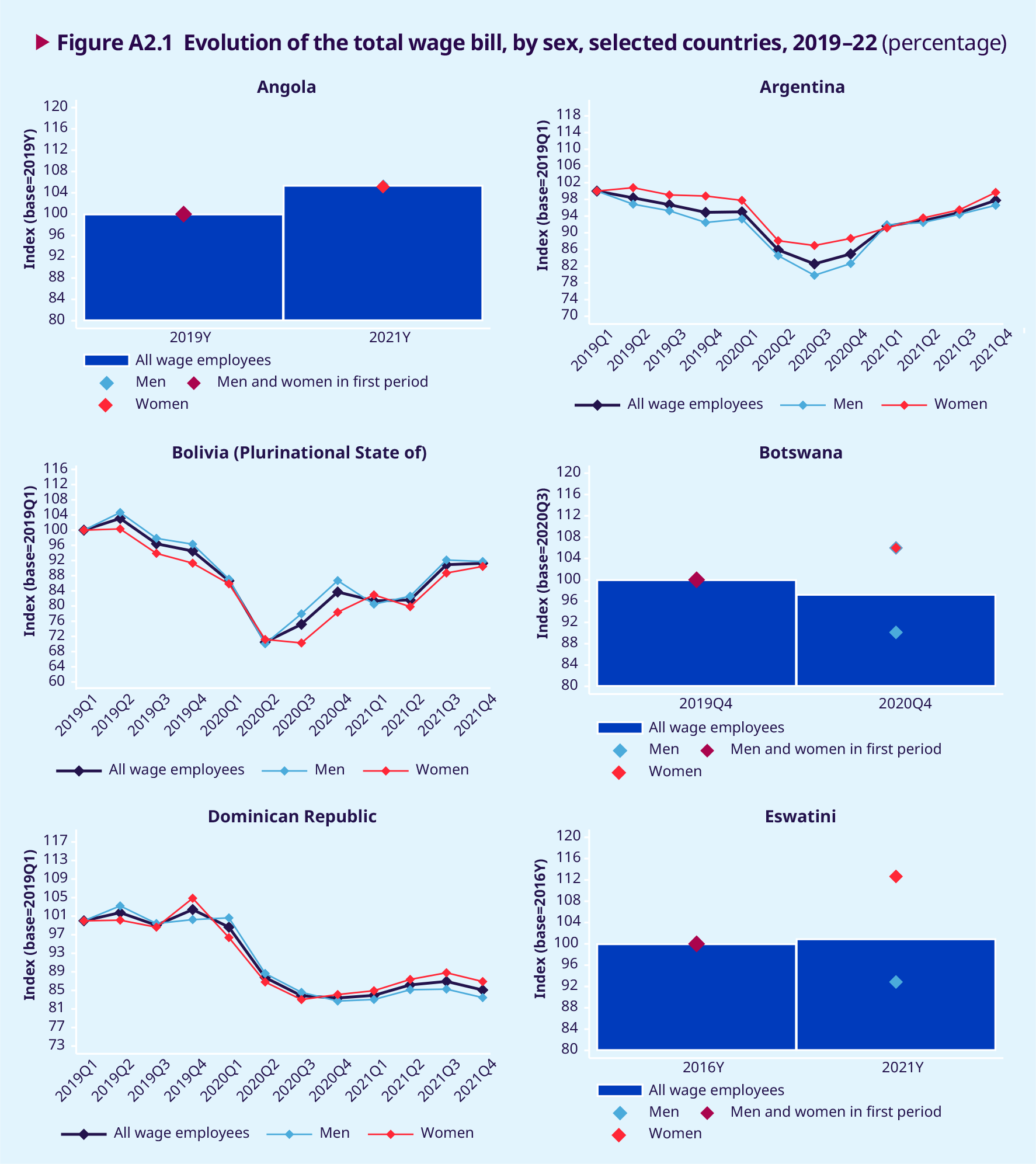
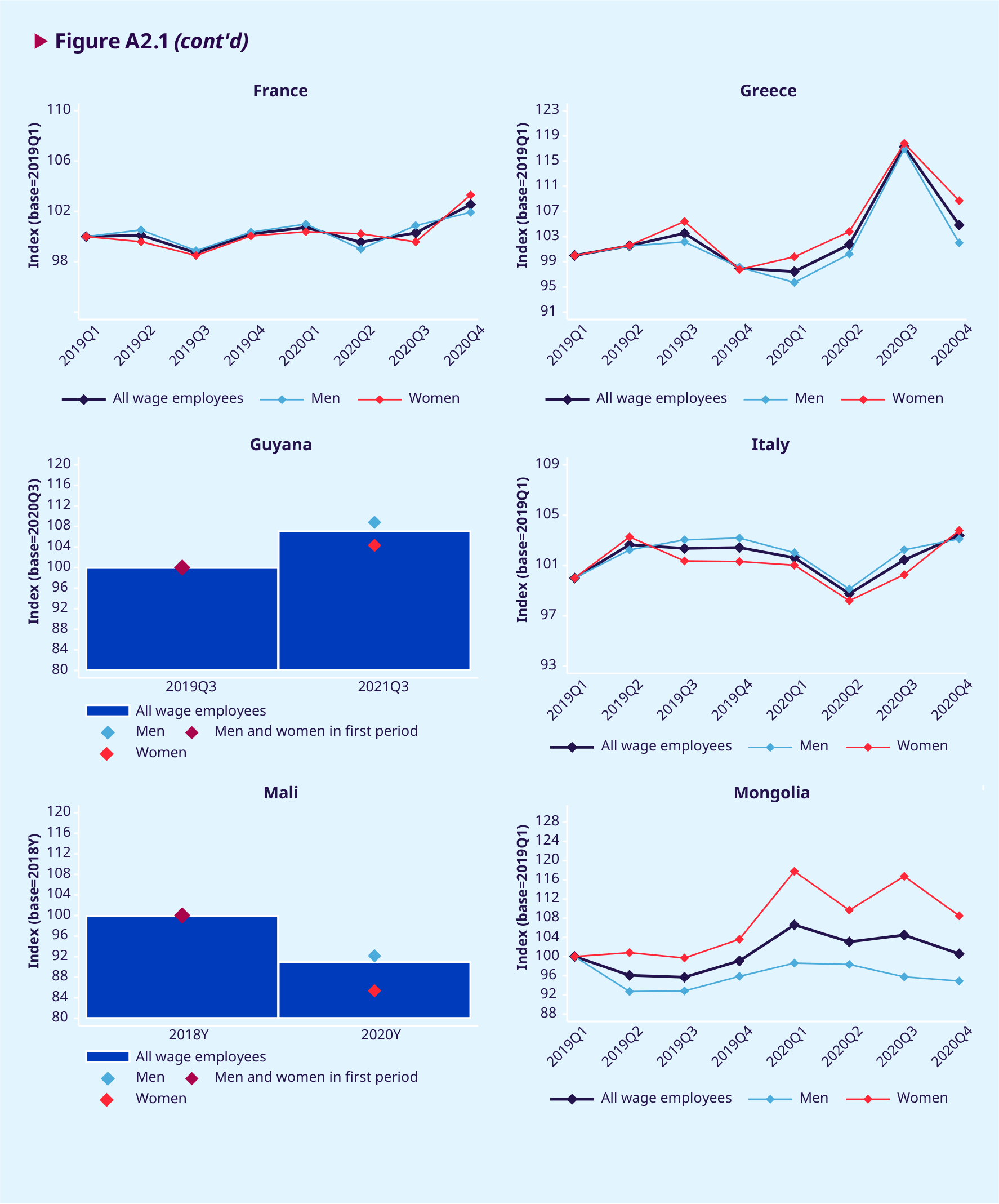
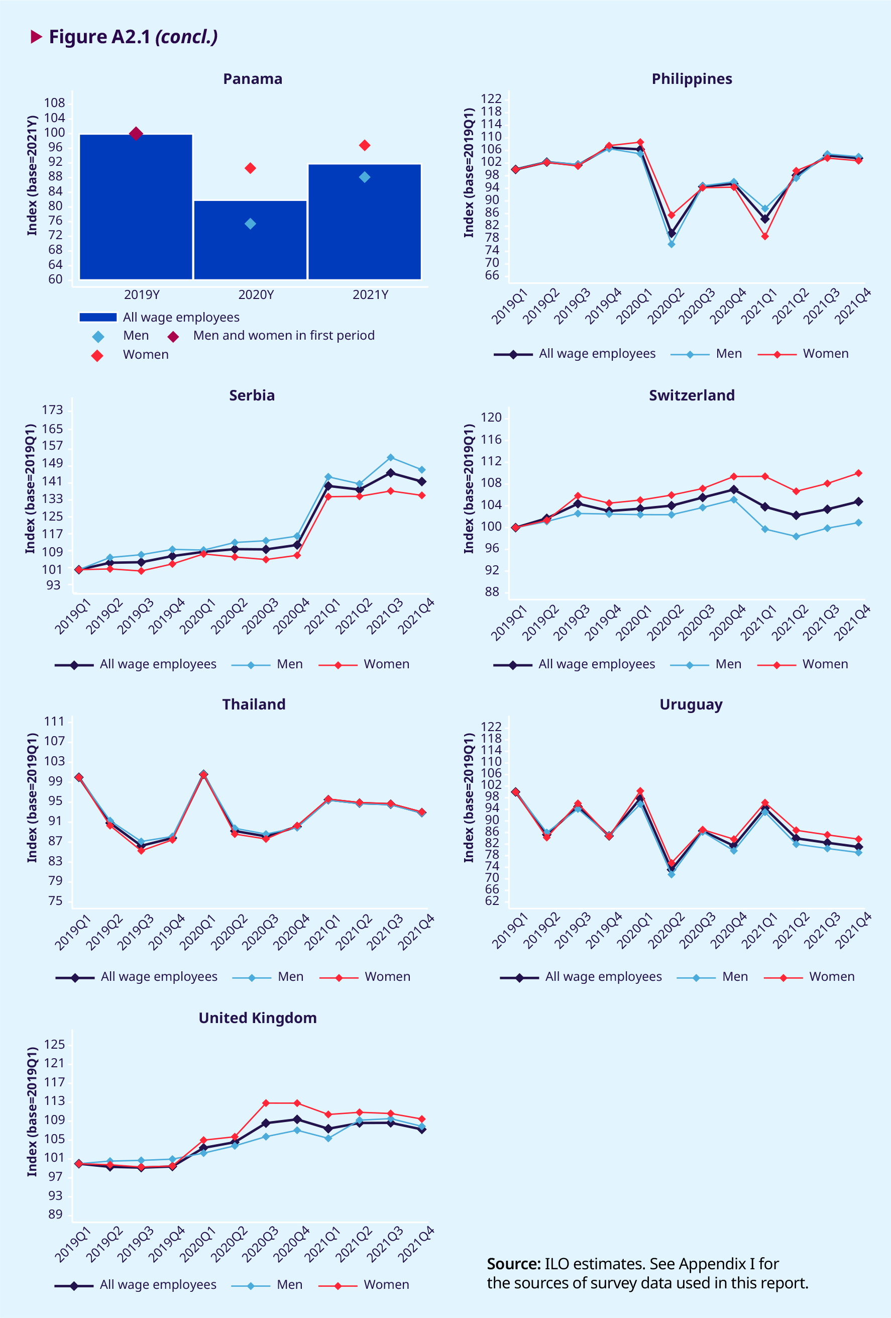
This appendix complements figure 3.12 in section 3.7. The charts below trace the evolution of the to- tal wage bill – for all wage employees, as well as for women and men separately – from the first quar- ter of 2019 up to the last available quarter in the data, which may be the last quarter of 2020, the last quarter of 2021 or the first or second quarter of 2022. The charts cover only countries that were not included in figure 3.12. They are bar charts if the frequency of the data is annual or irregular between quarters, and line graphs showing trends in all oth- er cases.

.Appendix III. Decomposing changes in the total wage bill and estimating changes in employment and earnings across the wage distribution

Decomposing the change in the total wage bill over time

The total wage bill for any given country is defined as the sum of total earnings generated by all wage employees in that country at some specific time. For example, if the total number of wage employees in country Z in January of year Y is 1 million and their average wage in January of that year is 100 local currency units, the total wage bill in country Z in January of year Y is 100 million local currency units. In generic terms, if EMP_t represents the total number of wage employees at time t for a given country, and represents the average (nominal or observed) earnings over the period between time 0 and time t (for example, over one year), the total wage bill, TWP_t, in nominal terms at time t in that country is given by the following equation:

$TW{B}_t=EM{P}_t\cdot w_t^n$ (1)

Equation (1) can be used to estimate the change in the total nominal-wage bill between a base period (time 0) and time t. For example, the change in the total wage bill in 2021 for any country relative to its total wage bill in 2019 (the base year) would be given by:

$\Delta TW{B}_{0,t}^{\text{Nominal}}=\left\{\frac{EM{P}_t\cdot w_t^n-EM{P}_0\cdot w_0^n}{EM{P}_0\cdot w_0^n}\right\}$ (2)

Continuing with the above example, if the number of wage employees at time t remains the same as in the base year, but earnings at time t have increased to 110 local currency units, the total wage bill has, on average, increased by 10 per cent over the intervening period relative to the base year. In general, the change in the total wage bill expressed by equation (2) is the sum of three components: a contribution due to the change in the number of wage employees over the period up to time t ; a contribution due to the change in inflation over that period; and a contribution due to the change in nominal earnings over that period. If αt represents the nominal wage increase between time 0 and time t, and πt represents the increase in price levels between time 0 and time t, the relationship between nominal wages (wⁿ) and real wages (w ^R) over that period can be expressed as follows:

$w_t^R=w_t^n\cdot (1-{\pi }_t)$ And $w_t^n=w_0^n\cdot (1+{\alpha }_t)$

Therefore

$w_t^n=w_0^n\cdot \left(1+{\alpha }_t\right)$ (3)

Equation (3) provides a link between real and nominal earnings and, together with equation (2), can be used to obtain an equation for the change in the total wage bill in real terms between time 0 (the base period) and time t, namely:

$\Delta TW{B}_{0,t}^{\text{Real}}=\left\{\frac{\left\{(EM{P}_t-EM{P}_0)\cdot w_0^n\right\}+\left\{EM{P}_t\cdot {\alpha }_t\cdot w_0^n\right\}-\left\{EM{P}_t\cdot {\pi }_t\cdot (1+{\alpha }_t)\cdot w_0^n\right\}}{EM{P}_0\cdot w_0^n}\right\}$ (4)

Equation (4) shows that in decomposing the change in the total real-wage bill between some base year and a later year, the effect of inflation and nominal changes cannot be fully disentangled – or, to be more precise, the way that inflation impacts on the total wage bill also includes the effects of inflation on the nominal change expressed by αt. This term can be constructed using the following expression: ${\alpha }_t=(w_t^n/w_o^n)-1$ while ${\pi }_t=(CP{I}_t/CP{I}_0)-1$ where CPI _t is the consumer price index at time t. Using equation (4), we therefore proceeded as follows:

• On the basis of the monthly labour earnings of wage employees throughout the year we estimated the total wage bill in 2019 and used this as the benchmark for comparison when determining the changes in 2020, 2021 and 2022. In the case of 2022, data are available only up to the first or second quarter, and so the comparison was performed against the corresponding quarters of 2019.

• Since 2019 is the base year, the total wage bill in real or nominal terms for 2019 is likewise used as the baseline. For the other three years, the estimate of the total wage bill is adjusted for inflation. The total wage bill in 2019 is the denominator in the expression on the right side of equation (4).

• Estimates of each component of the expression on the right side of equation (4) identify the contributions due to employment, the nominal change and inflation to changes in the total wage bill.

The decomposition method described above was used to obtain the estimates presented in figures 3.13 and 3.14 in section 3.8, and Appendix II.

Decomposing the total wage bill across the wage distribution over time

Employment and earnings (nominal and real) can change differently over time at different locations of the wage distribution. These changes were estimated as follows:

• 1. Using the base year 2019, we ranked wage employees according to their monthly earnings and created j groups of equal size. For example, if these equally sized groups are quintiles, each will include 20 per cent of wage employees in the population and j will be equal to 5. Each group is associated with an upper and lower threshold of (real) monthly earnings.

  2. Once the thresholds have been estimated at the base year (2019), they can be used to divide the population of wage employees observed in follow-up surveys (monthly, quarterly or annual) but with the 2019 thresholds adjusted for inflation. For example, if in 2019 the lowest quintile earned between 10 and 100 local currency units, and inflation in 2020 was 1 per cent, the thresholds in 2020 for this lowest-paid group would be 10.1 and 101 local currency units.

  3. After obtaining thresholds for the subsequent years, we divided the population of wage employees in each year into j groups. We used real monthly earnings to identify who falls into each of the groups in subsequent years. In the base year, the groups are of equal size (for example, if j = 5 they are groups containing 20 per cent of wage employees each) but in subsequent years the size of each group can change. Therefore, after the base year the groups are named ordinally as lowest, second, third, fourth and top earners.

  4. For 2019, we estimated the total number of wage earners in each group, the average nominal wage and the average real wage.

  5. The change in employment was estimated for subsequent years by comparing each group’s share of total employment with the share of the corresponding group in 2019.

  6. The changes in nominal and real wages were estimated by comparing each group’s average wage in 2019, 2020 or 2021 with the average wage in the following year, that is, 2020, 2021 or 2022.

The method described above to estimate changes in employment and in nominal and real monthly wages was used to obtain the estimates presented in figure 3.15 and 3.16 in section 3.9.

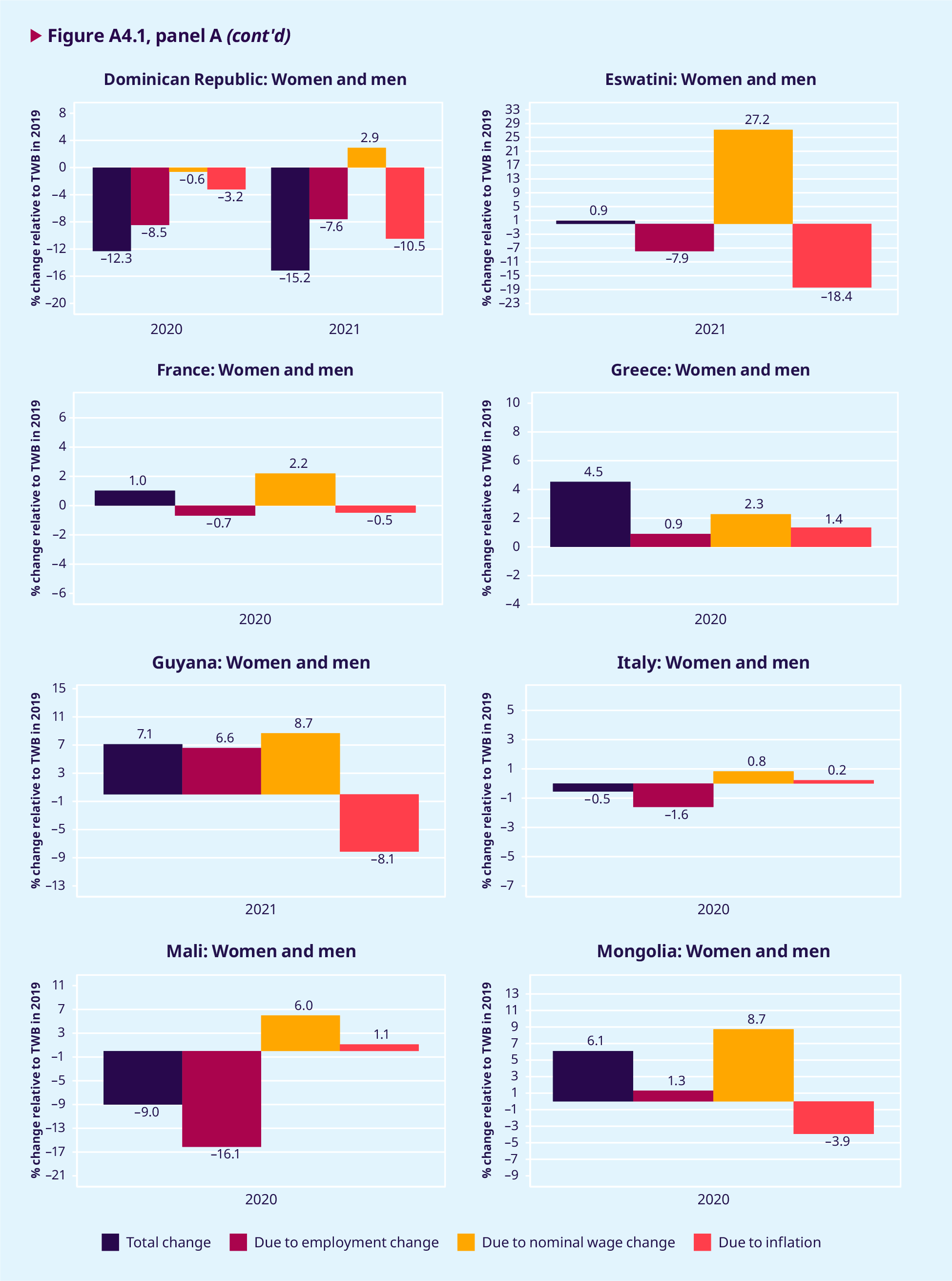
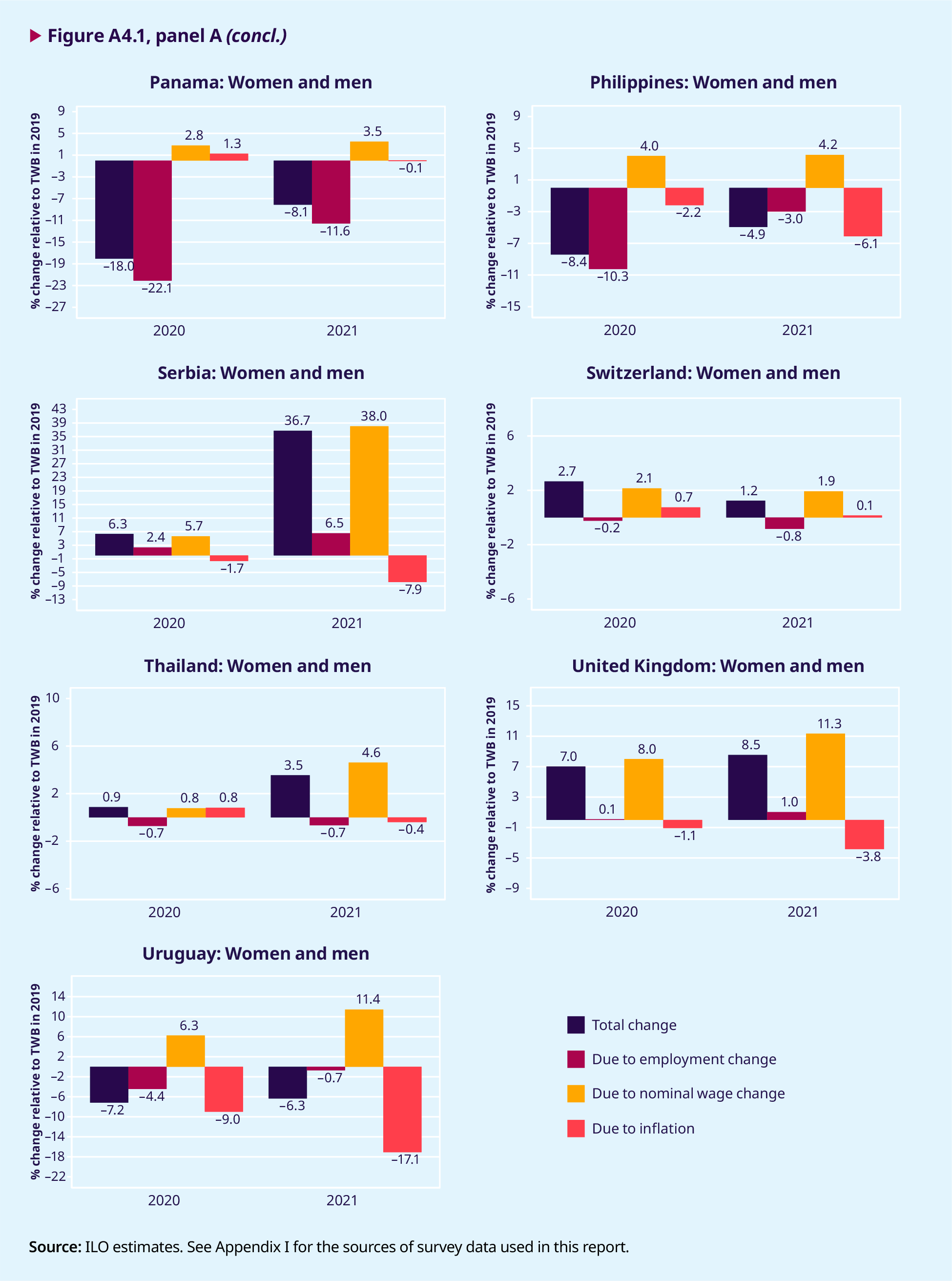
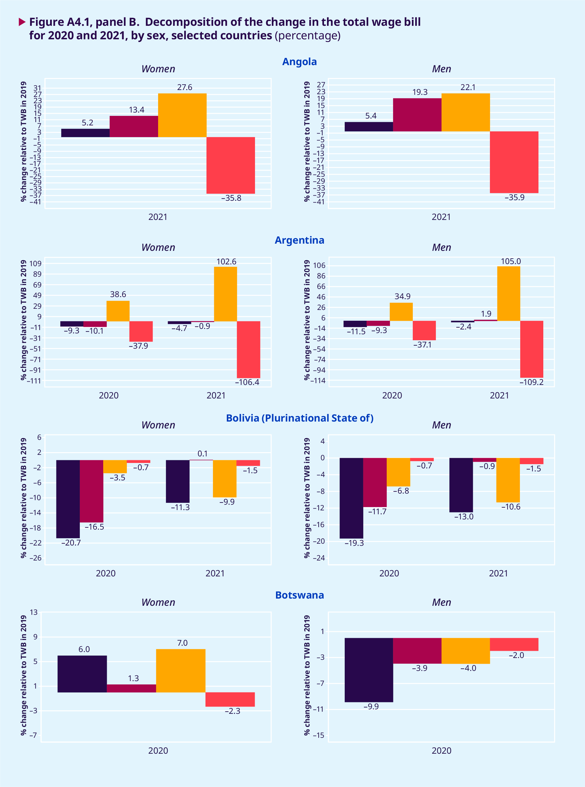
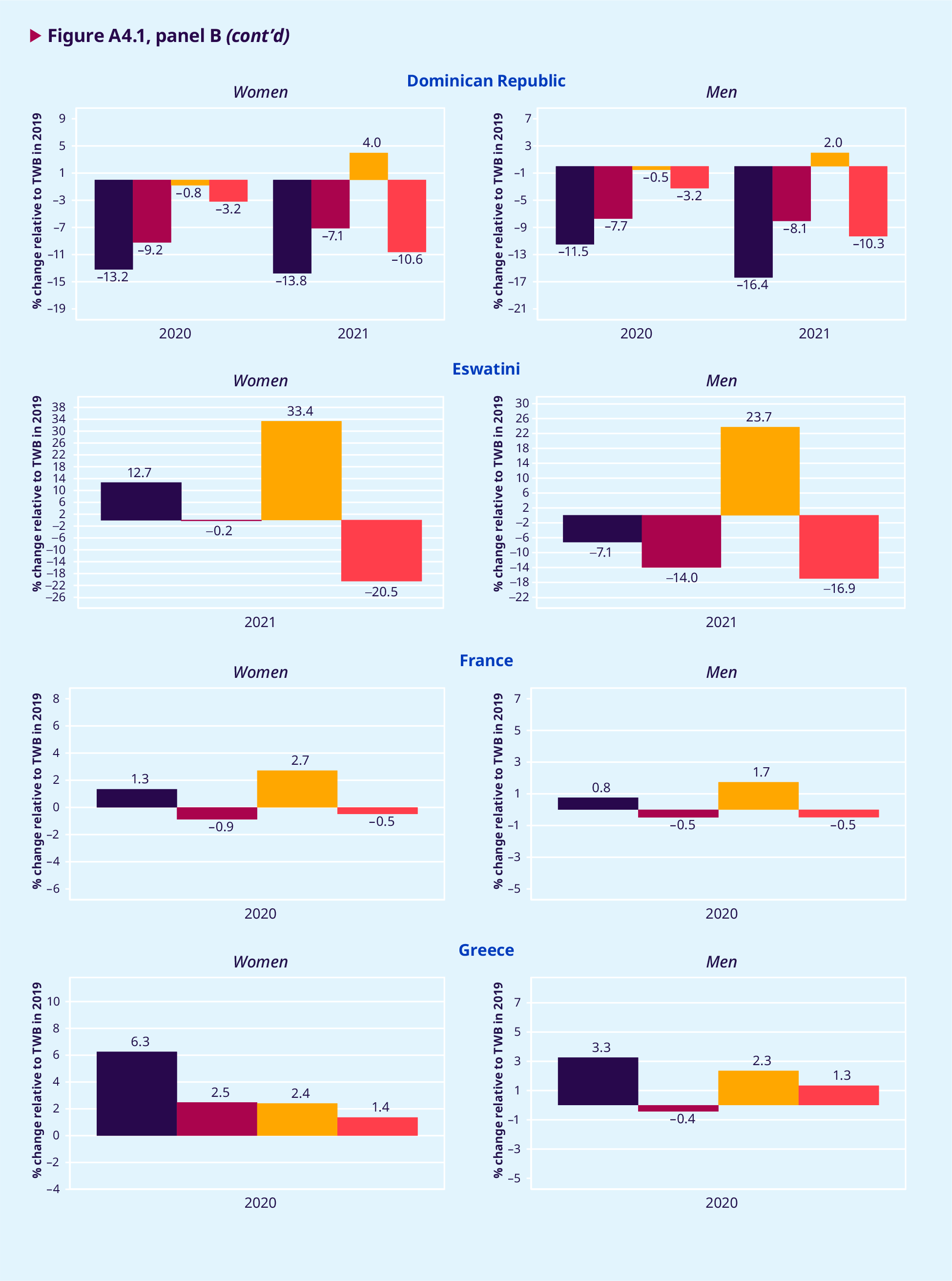
.Appendix IV. Decomposition of the change in the total wage bill for 2020 and 2021

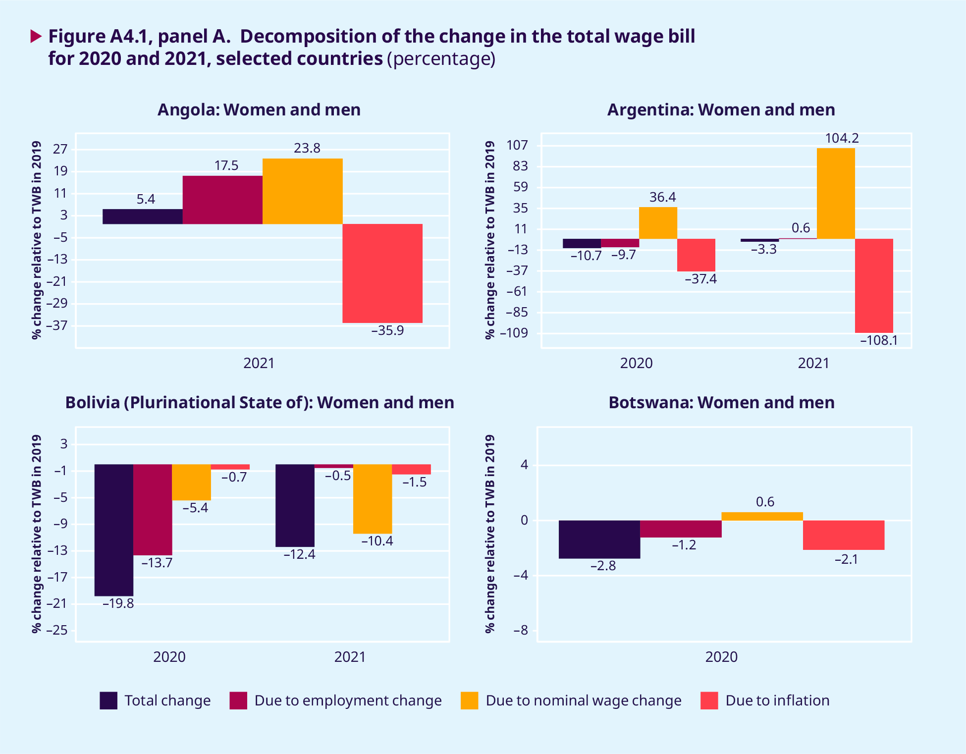
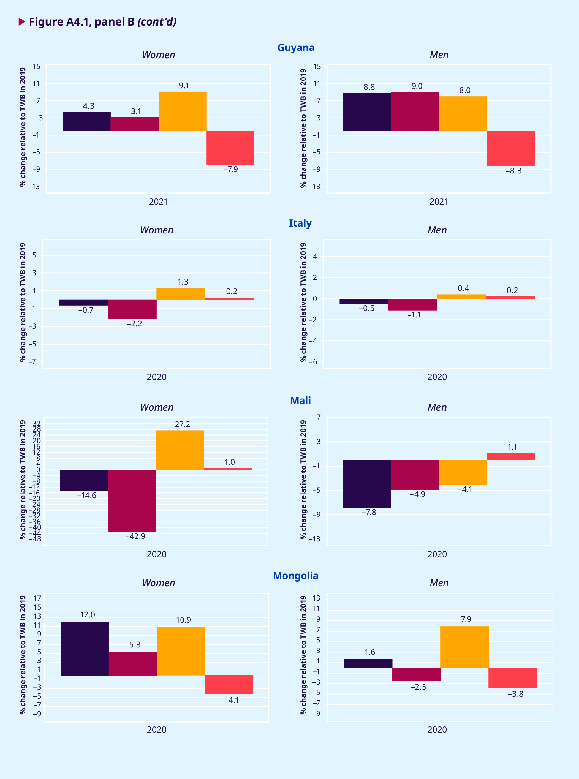
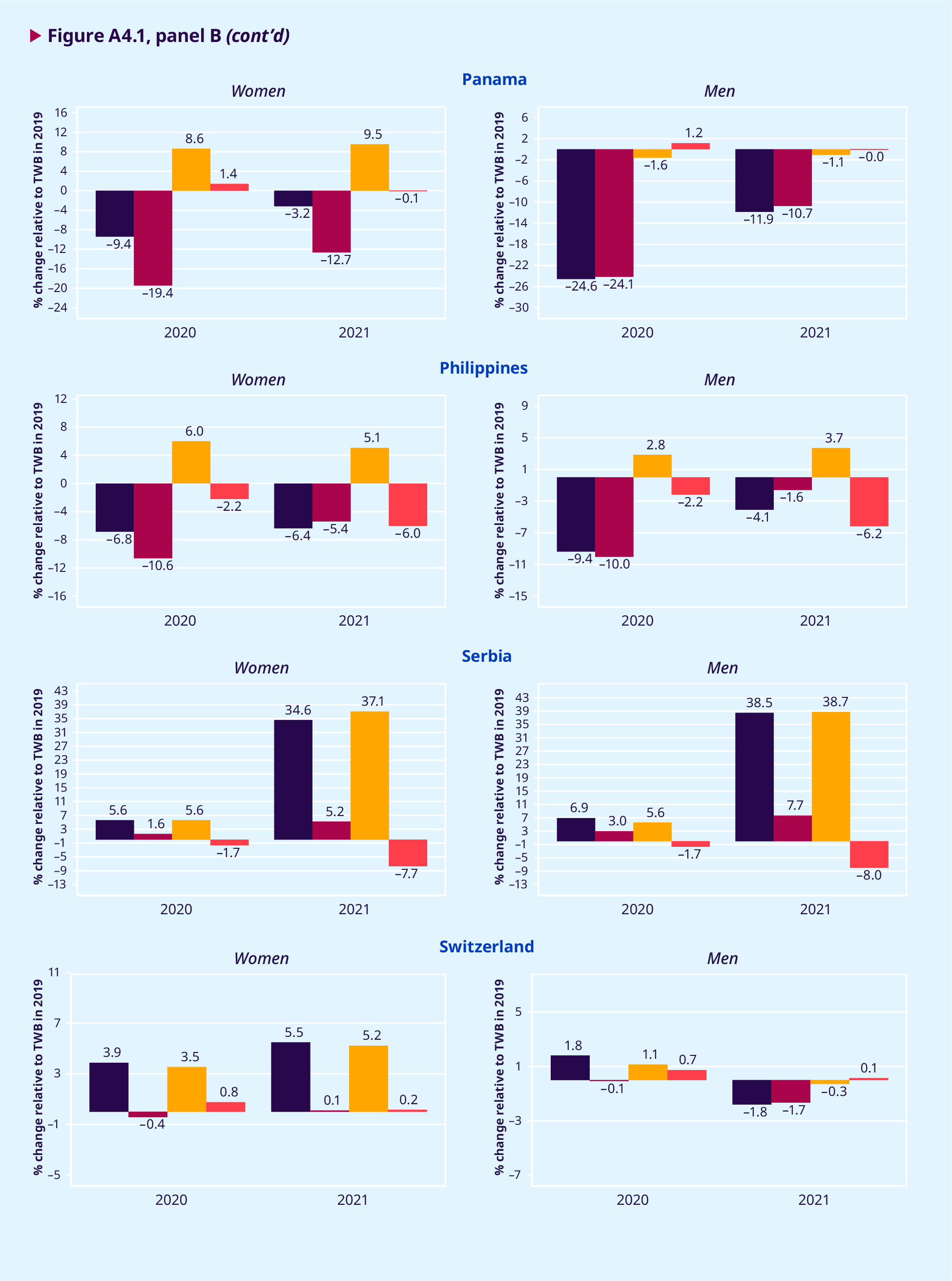
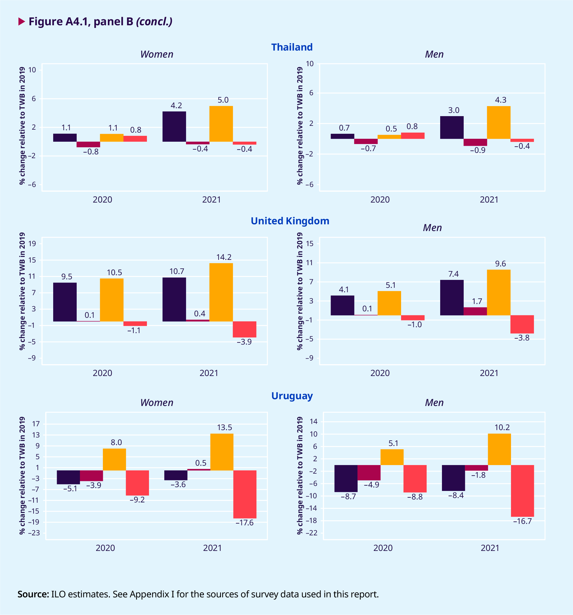
This appendix complements figures 3.13 and 3.14 in Chapter 3. The charts present a decomposition of the change in the total real-wage bill between 2019 and 2020, and between 2019 and 2021 (for countries that have already released data for 2021 at the time of writing). The decomposition shows the contributions to the change in the total wage bill (TWB) due to changes in total employment (including changes in the number of jobs and in the number of hours worked) and both real and nominal changes in hourly wages. Whereas the charts in figure A4.1, panel A, present a decomposition for all wage employees, panel B presents sex-disaggregated estimates. The charts in the two panels show only countries that were not included in figures 3.13 and 3.14.

.Appendix V. Decomposing the change in wage inequality over time

Section 4.2 of this report applies the method proposed by DiNardo, Fortin and Lemieux (1996) and further elaborated by Daly and Valletta (2006) to decompose changes in wage inequality between 2019 and 2021.1 In general, a change in wage inequality between two periods is the sum of a change in the composition of wage employees (for example, a change in the share of female wage employees) and a change in the wage structure (that is, a compression or widening of the wage scale, with the characteristics of wage employees held constant). Decomposition methods are useful in empirical labour economics because they allow one to distinguish between these two components.

The method proposed by DiNardo, Fortin and Lemieux (1996) involves comparing measures of wage inequality between two periods (for example, between 2019 and 2021) with the wage distribution in the later period (2021) adjusted to reflect the composition of wage employees from the earlier period (2019) while keeping the wage structure in the later period (2021) intact. The adjusted distribution is called the counterfactual wage distribution – that is, the distribution that would have been observed in 2021 in the absence of changes in the composition of wage employees relative to 2019. Since the counterfactual distribution emulates the 2019 composition of wage employees – thereby keeping the wage structure in 2021 intact – a comparison of the wage distribution in 2021 with the counterfactual distribution reveals the contribution that changes in the composition of wage employees have made to changes in wage inequality between 2019 and 2021. Likewise, since the counterfactual emulates the composition of wage employees in 2019, any difference between the counterfactual wage distribution and the wage distribution in 2019 reveals the contribution of structural changes to wage inequality. In short, the proposed decomposition method involves constructing a counterfactual wage distribution (for 2021) that emulates the composition of wage employees in 2019 (the pre-pandemic year) to disentangle the compositional and structural components that together make up the change in wage inequality observed between the two years. In what follows we explain: (a) how to construct the counterfactual wage distribution; and (b) how to use the proposed counterfactual to estimate the compositional and structural components of changes in wage inequality. Although in this report the counterfactual is based on the method proposed by DiNardo, Fortin and Lemieux (1996) there are other methods that are equally valid for this purpose. See Fortin, Lemieux and Firpo (2011) for a detailed account and comparison of various methods used to decompose measured outcomes in wage distributions.

Considering 2019 as the adjusting year, the counterfactual wage distribution for 2021 is the wage distribution that would have been observed in 2021 if the composition of wage employees in 2021 had remained the same as in 2019. Let $F(w,m_{2019}|t=2019)$ and $F(w,m_{2021}|t=2021)$ represent the wage distributions in 2019 and 2021, respectively, conditional on characteristics , where the suffix t denotes the year. For example, one characteristic in the set $m_t$ can be sex. Following DiNardo, Fortin and Lemieux (1996), we use “re-weighting” functions so that the composition of wage employees observed in 2019 (that is, $m_{2019}$ ) is imposed on the wage distribution observed in 2021 while keeping the wage structure in 2021 (that is, $F\left(w\right|t=2021)$) intact. Continuing with sex as the example characteristic, let us assume that women wage employees make up 48 per cent of the total population of wage employees in 2019 and that in 2021 they make up 40 per cent. Men wage employees would account for 52 per cent and 60 per cent in 2019 and 2021, respectively. A re- weighting function so that the gender composition in 2019 prevails in the 2021 wage distribution would be one that weights each woman observed in 2021 by the ratio 48/40 and each man by the ratio 52/60. Assuming that sex is the only variable in the set , the result of re-weighting women and men in 2021 according to their composition in 2019 results in a counterfactual wage distribution for 2021 that has the composition (of women and men) of 2019 but keeps the wage structure of 2021 intact. This counterfactual distribution can be expressed as $F(w,m_{2019}|t=2021)$. By comparing measures of wage inequality between $F(w,m_{2021}|t=2021)$ and $F(w,m_{2019}|t=2021)$ we can uncover the changes in wage inequality between the two years due to composition effects, while a comparison of measures of wage inequality between $F(w,m_{2019}|t=2021)$ and $F(w,m_{2019}|t=2019)$ reveals the changes in wage inequality between the two years due to changes in the wage structure.

In practice, the set $m_t$ $$ includes several variables which together describe the characteristics of wage employees (for example, sex, age and education); their working conditions (for example, contractual arrangements, occupational category, hours worked, and formal versus informal employment); and workplace attributes (for example, geographical location, economic sector and institutional sector). At the same time, the re-weighting functions are not ratios as in the simple example above: they are, rather, the outcomes of estimating conditional probability functions that take into account the categorical nature of variables when imposing their 2019 distribution on the wage distribution of 2021. For example, in the case of sex – a variable with only two categories – a logit specification can be used to estimate the conditional probability of being a woman ($\widehat{p}(g=1|s_t)$) or a man (1–$\widehat{p}(g=1|s_t)$ ) in 2019 and 2021, respectively, where the conditional includes all variables in $m_t$ except the variable “sex”. Using this example, the re-weighting function to adjust the wage distribution in 2021 so that it emulates the gender composition in 2019 would be constructed as: ${\psi }_{g=1}=\widehat{p}(g=1|s_{2019})/\widehat{p}(g=1\left|s_{2021}\right)$ for women and ${\psi }_{g=0}=\widehat{p}(g=0|s_{2019})/\widehat{p}(g=0\left|s_{2021}\right)$ for men, with $g_t=1$ and $g_t=0$ identifying women and men in each of the two years, respectively. Whereas the variable “sex” has only two categories, other variables may have several. For example, the variable “occupation” distinguishes several categories, from managers, professionals and technicians to semi-skilled, lower- skilled and unskilled occupations. When a variable has multiple categories, a multinomial logit model can be used to estimate the conditional probability of belonging to each category: the re-weighting function to impose the composition of a categorical variable with possible categories is constructed as for any categorical variable . Daly and Valletta (2006) extended the method of DiNardo, Fortin and Lemieux (1996) to cover categorical variables using multinomial (logit) specifications.

Imposing the composition of wage employees in 2019 on 2021 requires the estimation of re-weighting functions to account for all variables in the conditional $m_t$ set : these would include all the variables thought to be important in the wage determination process in both periods. Multiplying the (survey-provided) frequency weights by the re-weighting functions produces newly adjusted weights so that wage employees in 2021 emulate the composition of wage employees in 2019. Thus, if $f_{2019}\left(w\right)$ is the conditional density function for wages in 2019 and $f_{2021}\left(w\right)$ the conditional density function for wages in 2021, $f_{2021}^c\left(w\right)$ is the counterfactual conditional density function for wages in 2021 estimated using the newly adjusted frequency weights. Measures of wage inequality can be estimated from each of these three density functions: for example, the ratios between top and bottom deciles, which in logarithmic form can be expressed as $\Delta \mathrm{9,1}=Q9-Q1$ . Using $\Delta \mathrm{9,1}$ as an indicator of wage inequality, each of the three density functions can produce the corresponding measures: , $\Delta 9,1_{21}=Q{9}_{21}-Q{1}_{21}$, $\Delta 9,1_{19}=Q{9}_{19}-Q{1}_{19}$ and $\Delta 9,1_{21}^c=Q{9}_{21}^c-Q{1}_{21}^c$ – where the suffix 19 and 21 make references to years 2019 and 2021, respectively. The change in wage inequality between 2019 and 2021 for $\Delta \mathrm{9,1}$, that is, $\Delta 9,1_{t=\mathrm{19,21}}$ , can be expressed as follows:

$\Delta 9,1_{t=\mathrm{19,21}}=\left(Q{9}_{21}-Q{1}_{21}\right)-\left[Q{9}_{21}^c-Q{1}_{21}^c\right]+\left[Q{9}_{21}^c-Q{1}_{21}^c\right]-\left(Q{9}_{19}-Q{1}_{19}\right)$

->$\Delta 9,1_{t=\mathrm{19,21}}=\underset{COMPOSITION\hspace{0.33em}\hspace{0.33em}EFFECT}{\underbrace{\left(Q{9}_{21}-Q{9}_{21}^c\right)-\left(Q{1}_{21}-Q{1}_{21}^c\right)}}+\underset{STRUCTURAL\hspace{0.33em}\hspace{0.33em}EFFECT}{\underbrace{\left(Q{9}_{21}^c-Q{9}_{19}\right)-\left(Q{1}_{21}^c-Q{1}_{19}\right)}}$ (1)

Equation (1) shows the outcome of a counterfactual with all re-weighting functions applied to obtain $f_{2021}^c\left(w\right)$. In practice, the method proposed in DiNardo, Fortin and Lemieux (1996) makes it possible to identify the separate contributions of different factors in the composition of wage employees to the overall change in wage inequality between two periods. In section 4.2 of the report, the contributions to changing wage inequality due to compositional changes related to the following variables are identified in turn: sex, economic sector, occupational category and, lastly, “all other remaining factors”. The method is path-dependent, which means that the contribution of each component in the composition effect to the overall change in wage inequality can vary depending on the order in which the re-weighting function is updated to obtain the final estimate of the counterfactual wage distribution. See DiNardo, Fortin and Lemieux (1996) for further details.